|
\(\begin{matrix}
f_{0}
\'"`UNIQ-MathJax4-QINU`"'
Here, \(\mathrm{d}A_i\) is a set of two differential propositions, \(\mathrm{d}A_i = \{(\mathrm{d}a_i), \mathrm{d}a_i\},\) where \((\mathrm{d}a_i)\) is a proposition with the logical value of "\(\text{not}\ \mathrm{d}a_i\)". Each component \(\mathrm{d}A_i\) has the type \(\mathbb{B},\) operating under the ordered correspondence \(\{(\mathrm{d}a_i), \mathrm{d}a_i\} \cong \{0, 1\}.\) However, clarity is often served by acknowledging this differential usage with a superficially distinct type \(\mathbb{D},\) whose intension may be indicated as follows:
\[\mathbb{D} = \{(\mathrm{d}a_i), \mathrm{d}a_i\} = \{\text{same}, \text{different}\} = \{\text{stay}, \text{change}\} = \{\text{stop}, \text{step}\}.\]
Viewed within a coordinate representation, spaces of type \(\mathbb{B}^n\) and \(\mathbb{D}^n\) may appear to be identical sets of binary vectors, but taking a view at this level of abstraction would be like ignoring the qualitative units and the diverse dimensions that distinguish position and momentum, or the different roles of quantity and impulse.
An Interlude on the Path
|
|
There would have been no beginnings: instead, speech would proceed from me, while I stood in its path – a slender gap – the point of its possible disappearance.
|
|
| — Michel Foucault, The Discourse on Language, [Fou, 215]
|
A sense of the relation between \(\mathbb{B}\) and \(\mathbb{D}\) may be obtained by considering the path classifier (or the equivalence class of curves) approach to tangent vectors. Consider a universe \([\mathcal{X}].\!\) Given the boolean value system, a path in the space \(X = \langle \mathcal{X} \rangle\) is a map \(q : \mathbb{B} \to X.\) In this context the set of paths \((\mathbb{B} \to X)\) is isomorphic to the cartesian square \(X^2 = X \times X,\) or the set of ordered pairs chosen from \(X.\!\)
We may analyze \(X^2 = \{ (u, v) : u, v \in X \}\) into two parts, specifically, the ordered pairs \((u, v)\!\) that lie on and off the diagonal:
\[\begin{matrix}
X^2 & = & \{ (u, v) : u = v \} & \cup & \{ (u, v) : u \ne v \}.
\end{matrix}\]
This partition may also be expressed in the following symbolic form:
\[\begin{matrix}
X^2 & \cong & \mathrm{diag}(X) & + & 2 \tbinom{X}{2}.
\end{matrix}\]
The separate terms of this formula are defined as follows:
\[\begin{matrix}
\mathrm{diag}(X) & = & \{ (x, x) : x \in X \}.
\end{matrix}\!\]
\[\begin{matrix}
\tbinom{X}{k} & = & X\ \mathrm{choose}\ k & = & \{ k\!\text{-sets from}\ X \}.
\end{matrix}\!\]
Thus we have:
\[\begin{matrix}
\tbinom{X}{2} & = & \{ \{ u, v \} : u, v \in X \}.
\end{matrix}\]
We may now use the features in \(\mathrm{d}\mathcal{X} = \{ \mathrm{d}x_i \} = \{ \mathrm{d}x_1, \ldots, \mathrm{d}x_n \}\) to classify the paths of \((\mathbb{B} \to X)\) by way of the pairs in \(X^2.\!\) If \(X \cong \mathbb{B}^n,\) then a path \(q\!\) in \(X\!\) has the following form:
\[\begin{matrix}
q : (\mathbb{B} \to \mathbb{B}^n) & \cong & \mathbb{B}^n \times \mathbb{B}^n & \cong & \mathbb{B}^{2n} & \cong & (\mathbb{B}^2)^n.
\end{matrix}\]
Intuitively, we want to map this \((\mathbb{B}^2)^n\) onto \(\mathbb{D}^n\) by mapping each component \(\mathbb{B}^2\) onto a copy of \(\mathbb{D}.\) But in the presenting context "\(\mathbb{D}\)" is just a name associated with, or an incidental quality attributed to, coefficient values in \(\mathbb{B}\) when they are attached to features in \(\mathrm{d}\mathcal{X}.\)
Taking these intentions into account, define \(\mathrm{d}x_i : X^2 \to \mathbb{B}\) in the following manner:
\(\begin{array}{lcrcl}
\mathrm{d}x_i ((u, v)) & = & (\!|\ x_i (u) & , & x_i (v)\ |\!) \\
& = & x_i (u) & + & x_i (v) \\
& = & x_i (v) & - & x_i (u). \\
\end{array}\)
In the above transcription, the operator bracket of the form \((\!| \ldots\ ,\ \ldots |\!)\) is a cactus lobe, in general signifying that just one of the arguments listed is false. In the case of two arguments this is the same thing as saying that the arguments are not equal. The plus sign signifies boolean addition, in the sense of addition in \(\mathrm{GF}(2),\) and thus means the same thing in this context as the minus sign, in the sense of adding the additive inverse.
The above definition of \(\mathrm{d}x_i : X^2 \to \mathbb{B}\) is equivalent to defining \(\mathrm{d}x_i : (\mathbb{B} \to X) \to \mathbb{B}\!\) in the following way:
\(\begin{array}{lcrcl}
\mathrm{d}x_i (q) & = & (\!|\ x_i (q_0) & , & x_i (q_1)\ |\!) \\
& = & x_i (q_0) & + & x_i (q_1) \\
& = & x_i (q_1) & - & x_i (q_0). \\
\end{array}\)
In this definition \(q_b = q(b),\!\) for each \(b\!\) in \(\mathbb{B}.\) Thus, the proposition \(\mathrm{d}x_i\) is true of the path \(q = (u, v)\!\) exactly if the terms of \(q,\!\) the endpoints \(u\!\) and \(v,\!\) lie on different sides of the question \(x_i.\!\)
The language of features in \(\langle \mathrm{d}\mathcal{X} \rangle,\) indeed the whole calculus of propositions in \([\mathrm{d}\mathcal{X}],\) may now be used to classify paths and sets of paths. In other words, the paths can be taken as models of the propositions \(g : \mathrm{d}X \to \mathbb{B}.\) For example, the paths corresponding to \(\mathrm{diag}(X)\) fall under the description \((\!| \mathrm{d}x_1 |\!) \cdots (\!| \mathrm{d}x_n |\!),\) which says that nothing changes against the backdrop of the coordinate frame \(\{ x_1, \ldots, x_n \}.\)
Finally, a few words of explanation may be in order. If this concept of a path appears to be described in a roundabout fashion, it is because I am trying to avoid using any assumption of vector space properties for the space \(X\!\) that contains its range. In many ways the treatment is still unsatisfactory, but improvements will have to wait for the introduction of substitution operators acting on singular propositions.
The Extended Universe of Discourse
|
|
At the moment of speaking, I would like to have perceived a nameless voice, long preceding me, leaving me merely to enmesh myself in it, taking up its cadence, and to lodge myself, when no one was looking, in its interstices as if it had paused an instant, in suspense, to beckon to me.
|
|
| — Michel Foucault, The Discourse on Language, [Fou, 215]
|
Next we define the extended alphabet or bundled alphabet \(\mathrm{E}\mathcal{A}\) as follows:
\(\begin{array}{lclcl}
\mathrm{E}\mathcal{A}
& = & \mathcal{A} \cup \mathrm{d}\mathcal{A}
& = & \{a_1, \ldots, a_n, \mathrm{d}a_1, \ldots, \mathrm{d}a_n\}. \\
\end{array}\)
This supplies enough material to construct the differential extension \(\mathrm{E}A,\) or the tangent bundle over the initial space \(A,\!\) in the following fashion:
\(\begin{array}{lcl}
\mathrm{E}A
& = & \langle \mathrm{E}\mathcal{A} \rangle \\
& = & \langle \mathcal{A} \cup \mathrm{d}\mathcal{A} \rangle \\
& = & \langle a_1, \ldots, a_n, \mathrm{d}a_1, \ldots, \mathrm{d}a_n \rangle, \\
\end{array}\)
and also:
\(\begin{array}{lcl}
\mathrm{E}A
& = & A \times \mathrm{d}A \\
& = & A_1 \times \ldots \times A_n \times \mathrm{d}A_1 \times \ldots \times \mathrm{d}A_n. \\
\end{array}\)
This gives \(\mathrm{E}A\) the type \(\mathbb{B}^n \times \mathbb{D}^n.\)
Finally, the tangent universe \(\mathrm{E}A^\circ = [\mathrm{E}\mathcal{A}]\!\) is constituted from the totality of points and maps, or interpretations and propositions, that are based on the extended set of features \(\mathrm{E}\mathcal{A},\) and this fact is summed up in the following notation:
\(\begin{array}{lclcl}
\mathrm{E}A^\circ
& = & [\mathrm{E}\mathcal{A}]
& = & [a_1, \ldots, a_n, \mathrm{d}a_1, \ldots, \mathrm{d}a_n]. \\
\end{array}\)
This gives the tangent universe \(\mathrm{E}A^\circ\!\) the type:
\(\begin{array}{lcl}
(\mathbb{B}^n \times \mathbb{D}^n\ +\!\to \mathbb{B})
& = & (\mathbb{B}^n \times \mathbb{D}^n, (\mathbb{B}^n \times \mathbb{D}^n \to \mathbb{B})). \\
\end{array}\)
A proposition in the tangent universe \([\mathrm{E}\mathcal{A}]\) is called a differential proposition and forms the analogue of a system of differential equations, constraints, or relations in ordinary calculus.
With these constructions, the differential extension \(\mathrm{E}A\) and the space of differential propositions \((\mathrm{E}A \to \mathbb{B}),\!\) we have arrived, in main outline, at one of the major subgoals of this study. Table 8 summarizes the concepts that have been introduced for working with differentially extended universes of discourse.
\(\text{Table 8.} ~~ \text{Differential Extension : Basic Notation}\!\)
| \(\text{Symbol}\!\)
|
\(\text{Notation}\!\)
|
\(\text{Description}\!\)
|
\(\text{Type}\!\)
|
| \(\mathrm{d}\mathfrak{A}\!\)
|
\(\{ {}^{\backprime\backprime} \mathrm{d}a_1 {}^{\prime\prime}, \ldots, {}^{\backprime\backprime} \mathrm{d}a_n {}^{\prime\prime} \}\!\)
|
\(\begin{matrix}
\text{Alphabet of}
\'"`UNIQ-MathJax12-QINU`"'
On formal occasions, such as the present context of definition, the tacit extension from \(\mathcal{X}\) to \(\mathcal{Y}\) is explicitly symbolized by the operator \(\epsilon : (\langle \mathcal{X} \rangle \to \mathbb{B}) \to (\langle \mathcal{Y} \rangle \to \mathbb{B}),\) where the appropriate alphabets \(\mathcal{X}\) and \(\mathcal{Y}\) are understood from context, but normally one may leave the "\(\epsilon\!\)" silent.
Let's explore what this means for the present Example. Here, \(\mathcal{X} = \{ A \}\) and \(\mathcal{Y} = \mathrm{E}\mathcal{X} = \{ A, \mathrm{d}A \}.\) For each of the propositions \(f_i\!\) over \(X\!,\) specifically, those whose expression \(e_i\!\) lies in the collection \(\{ 0, (A), A, 1 \},\!\) the tacit extension \(\epsilon f\!\) of \(f\!\) to \(\mathrm{E}X\) can be phrased as a logical conjunction of two factors, \(f_i = e_i \cdot \tau\ ,\) where \(\tau\!\) is a logical tautology that uses all the variables of \(\mathcal{Y} - \mathcal{X}.\) Working in these terms, the tacit extensions \(\epsilon f\!\) of \(f\!\) to \(\mathrm{E}X\) may be explicated as shown in Table 15.
\(\text{Table 15.}~~\text{Tacit Extension of}~ [A] ~\text{to}~ [A, \mathrm{d}A]\!\)
|
|
\(0\!\)
|
\(=\!\)
|
\(0\!\)
|
\(\cdot\!\)
|
\(((\mathrm{d}A) ~,~ \mathrm{d}A)\!\)
|
\(=\!\)
|
\(0\!\)
|
|
|
|
\((A)\!\)
|
\(=\!\)
|
\((A)\!\)
|
\(\cdot\!\)
|
\(((\mathrm{d}A) ~,~ \mathrm{d}A)\!\)
|
\(=\!\)
|
\((A)(\mathrm{d}A) ~+~ (A)~\mathrm{d}A\!\)
|
|
|
|
\(A\!\)
|
\(=\!\)
|
\(A\!\)
|
\(\cdot\!\)
|
\(((\mathrm{d}A) ~,~ \mathrm{d}A)\!\)
|
\(=\!\)
|
\(A~(\mathrm{d}A) ~+~ A~\mathrm{d}A\!\)
|
|
|
|
\(1\!\)
|
\(=\!\)
|
\(1\!\)
|
\(\cdot\!\)
|
\(((\mathrm{d}A) ~,~ \mathrm{d}A)\!\)
|
\(=\!\)
|
\(1\!\)
|
|
In its effect on the singular propositions over \(X,\!\) this analysis has an interesting interpretation. The tacit extension takes us from thinking about a particular state, like \(A\!\) or \((A),\!\) to considering the collection of outcomes, the outgoing changes or the singular dispositions, that spring from that state.
Example 2. Drives and Their Vicissitudes
|
|
I open my scuttle at night and see the far-sprinkled systems,
And all I see, multiplied as high as I can cipher, edge but
the rim of the farther systems.
|
|
|
— Walt Whitman, Leaves of Grass, [Whi, 81]
|
Before we leave the one-feature case let's look at a more substantial example, one that illustrates a general class of curves that can be charted through the extended feature spaces and that provides an opportunity to discuss a number of important themes concerning their structure and dynamics.
Again, let X = {x1} = {A}. In the discussion that follows I will consider a class of trajectories having the property that dkA = 0 for all k greater than some fixed m, and I indulge in the use of some picturesque terms that describe salient classes of such curves. Given the finite order condition, there is a highest order non-zero difference dmA exhibited at each point in the course of any determinate trajectory that one may wish to consider. With respect to any point of the corresponding orbit or curve let us call this highest order differential feature dmA the drive at that point. Curves of constant drive dmA are then referred to as "mth gear curves".
- Scholium. The fact that a difference calculus can be developed for boolean functions is well known [Fuji], [Koh, § 8-4] and was probably familiar to Boole, who was an expert in difference equations before he turned to logic. And of course there is the strange but true story of how the Turin machines of the 1840's prefigured the Turing machines of the 1940's [Men, 225-297]. At the very outset of general purpose, mechanized computing we find that the motive power driving the Analytical Engine of Babbage, the kernel of an idea behind all of his wheels, was exactly his notion that difference operations, suitably trained, can serve as universal joints for any conceivable computation [M&M], [Mel, ch. 4].
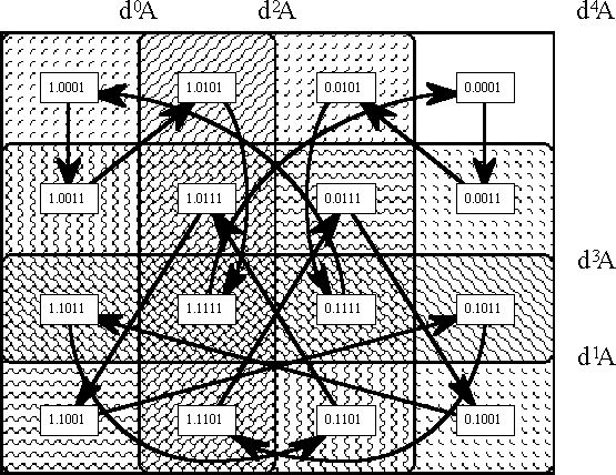
Given this language, the particular Example that I take up here can be described as the family of 4th gear curves through E4X = 〈A, dA, d2A, d3A, d4A〉. These are the trajectories generated subject to the dynamic law d4A = 1, where it is understood in such a statement that all higher order differences are equal to 0. Since d4A and all higher dkA are fixed, the temporal or transitional conditions (initial, mediate, terminal — transient or stable states) vary only with respect to their projections as points of E3X = 〈A, dA, d2A, d3A〉. Thus, there is just enough space in a planar venn diagram to plot all of these orbits and to show how they partition the points of E3X. It turns out that there are exactly two possible orbits, of eight points each, as illustrated in Figure 16.
|
|
| \(\text{Figure 16.} ~~ \text{A Couple of Fourth Gear Orbits}\!\)
|
With a little thought it is possible to devise an indexing scheme for the general run of dynamic states that allows for comparing universes of discourse that weigh in on different scales of observation. With this end in sight, let us index the states q in EmX with the dyadic rationals (or the binary fractions) in the half-open interval [0, 2). Formally and canonically, a state qr is indexed by a fraction r = s/t whose denominator is the power of two t = 2m and whose numerator is a binary numeral that is formed from the coefficients of state in a manner to be described next. The differential coefficients of the state q are just the values dkA(q), for k = 0 to m, where d0A is defined as being identical to A. To form the binary index d0.d1…dm of the state q the coefficient dkA(q) is read off as the binary digit dk associated with the place value 2–k. Expressed by way of algebraic formulas, the rational index r of the state q can be given by the following equivalent formulations:
| \(r(q)\!\)
|
\(=\!\)
|
\(\sum_k d_k \cdot 2^{-k}\!\)
|
\(=\!\)
|
\(\sum_k \text{d}^k A(q) \cdot 2^{-k}\!\)
|
| \(=\!\)
|
| \(\frac{s(q)}{t}\!\)
|
\(=\!\)
|
\(\frac{\sum_k d_k \cdot 2^{(m-k)}}{2^m}\!\)
|
\(=\!\)
|
\(\frac{\sum_k \text{d}^k A(q) \cdot 2^{(m-k)}}{2^m}\!\)
|
|
Applied to the example of fourth gear curves, this scheme results in the data of Tables 17-a and 17-b, which exhibit one period for each orbit. The states in each orbit are listed as ordered pairs ‹pi, qj›, where pi may be read as a temporal parameter that indicates the present time of the state, and where j is the decimal equivalent of the binary numeral s. Informally and more casually, the Tables exhibit the states qs as subscripted with the numerators of their rational indices, taking for granted the constant denominators of 2m = 24 = 16. Within this set-up, the temporal successions of states can be reckoned as given by a kind of parallel round-up rule. That is, if ‹dk, dk+1› is any pair of adjacent digits in the state index r, then the value of dk in the next state is dk′ = dk + dk+1.
\(\text{Table 17-a.} ~~ \text{A Couple of Orbits in Fourth Gear : Orbit 1}\!\)
| \(\text{Time}\!\)
|
\(\text{State}\!\)
|
\(A\!\)
|
\(\mathrm{d}A\)
|
|
|
|
| \(p_i\!\)
|
\(q_j\!\)
|
\(\mathrm{d}^0\!A\)
|
\(\mathrm{d}^1\!A\)
|
\(\mathrm{d}^2\!A\)
|
\(\mathrm{d}^3\!A\)
|
\(\mathrm{d}^4\!A\)
|
|
\(\begin{matrix}
p_0
\'"`UNIQ-MathJax13-QINU`"'''F'' : [''u''<sub>1</sub>, …, ''u''<sub>''n''</sub>, d''u''<sub>1</sub>, …, d''u''<sub>''n''</sub>] → [d''x''<sub>1</sub>, …, d''x''<sub>''k''</sub>]
which is defined by the equations:
<br><font face="courier new">
{| align="center" border="1" cellpadding="12" cellspacing="0" style="font-weight:bold; text-align:left; width:96%"
|
{| align="center" border="0" cellpadding="4" cellspacing="0" style="font-weight:bold; text-align:left; width:100%"
| width="8%" | d''x''<sub>1</sub>
| width="4%" | =
| width="44%" | \(\epsilon\)F1‹u1, …, un, du1, …, dun›
|
=
|
F1‹u1, …, un›
|
| ...
|
| dxk
|
=
|
\(\epsilon\)Fk‹u1, …, un, du1, …, dun›
|
=
|
Fk‹u1, …, un›
|
|
In effect, the operator \(\eta\) is nothing but the stand-alone version of a procedure that is otherwise invoked subordinate to the work of the radius operator e. Operating independently, \(\eta\) achieves precisely the same results that the second \(\epsilon\) in ‹\(\epsilon\), \(\epsilon\)› accomplishes by working within the context of its adjuvant thematic frame, "‹ , ›". From this point on, because the use of \(\epsilon\) and \(\eta\) in this setting combines the aims of both the tacit and the thematic extensions, and because \(\eta\) reflects in regard to \(\epsilon\) little more than the application of a differential twist, a mere turn of phrase, I refer to \(\eta\) as the trope extension operator.
The Chord Operator : D
|
|
What difference would it practically make to any one if this notion rather than that notion were true? If no practical difference whatever can be traced, then the alternatives mean practically the same thing, and all dispute is idle.
|
|
| — William James, Pragmatism, [Jam, 45]
|
Next I discuss an operator that is always immanent in this form of analysis, and remains implicitly present in the entire proceeding. It may appear once as a record: a relic or revenant that reprises the reminders of an earlier stage of development. Or it may appear always as a resource: a reserve or redoubt that caches in advance an echo of what remains to be played out, cleared up, and requited in full at a future stage. And all of this remains true whether or not we recall the key at any time, and whether or not the subtending theme is recited explicitly at any stage of play.
This is the operator that is referred to as r0 in the initial stage of analysis (Figure 33-i), and that is expanded as d1 + r1 in the subsequent step (Figure 33-ii). In congruence, but not quite harmony, with my allusions of analogy that are not quite geometry, I call this the chord operator and denote it D. In the more casual terms that are here introduced, D is defined as the remainder of E and e, and it assigns a due measure to each undertone of accord or discord that is struck between the note of enterprise E and the bar of exigency e.
The tension between these counterposed notions, in balance transient but regular in stridence, may be refracted along familiar lines, though never by any such fraction resolved. In this style we may write D = ‹\(\epsilon\), D›, calling D the difference operator and noting that it plays a role in this realm of mutable and diverse discourse that is analogous to the part taken by the discrete difference operator in the ordinary difference calculus. Finally, we should note that the chord D is not one that need be lost at any stage of development. At the mth stage of play it can always be reconstituted in the following form:
| D
|
=
|
E – e
|
|
|
=
|
r0
|
|
|
=
|
d1 + r1
|
|
|
=
|
d1 + … + dm + rm
|
|
|
=
|
∑(i = 1 … m) di + rm
|
|
The Tangent Operator : T
|
|
They take part in scenes of whose significance they have no inkling. They are merely tangent to curves of history the beginnings and ends and forms of which pass wholly beyond their ken. So we are tangent to the wider life of things.
|
|
| — William James, Pragmatism, [Jam, 300]
|
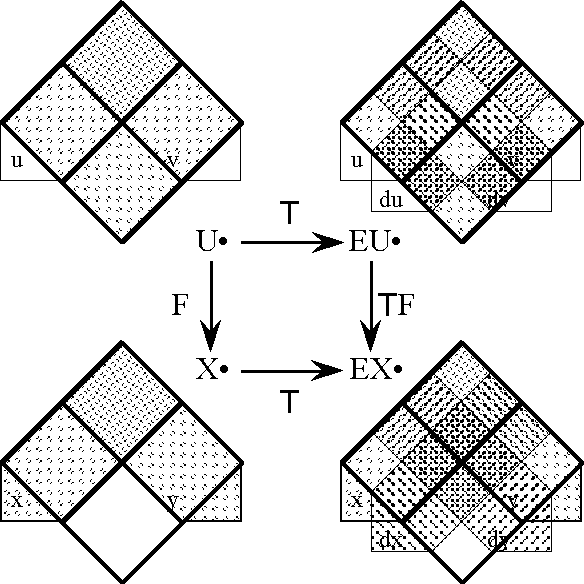
The operator tagged as d1 in the analytic diagram (Figure 33) is called the tangent operator, and is usually denoted in this text as d or T. Because it has the properties required to qualify as a functor, namely, preserving the identity element of the composition operation and the articulated form of every composure among transformations, it also earns the title of a tangent functor. According to the custom adopted here, we dissect it as T = d = ‹\(\epsilon\), d›, where d is the operator that yields the first order differential dF when applied to a transformation F, and whose name is legion.
Figure 34 illustrates a stage of analysis where we ignore everything but the tangent functor T, and attend to it chiefly as it bears on the first order differential dF in the analytic expansion of F. In this situation, we often refer to the extended universes EU • and EX • under the equivalent designations TU • and TX •, respectively. The purpose of the tangent functor T is to extract the tangent map TF at each point of U •, and the tangent map TF = ‹\(\epsilon\), d›F tells us not only what the transformation F is doing at each point of the universe U • but also what F is doing to states in the neighborhood of that point, approximately, linearly, and relatively speaking.
U%          $T$      $T$U%        $T$U%
   o------------------>o============o
   |                   |            |
   |                   |            |
   |                   |            |
   |                   |            |
F  |                   | $T$F   =   | <!e!, d> F
   |                   |            |
   |                   |            |
   |                   |            |
   v                   v            v
   o------------------>o============o
X%          $T$      $T$X%        $T$X%

Figure 34.  Tangent Functor Diagram
- NB. There is one aspect of the preceding construction that remains especially problematic. Why did we define the operators W in {\(\eta\), E, D, d, r} so that the ranges of their resulting maps all fall within the realms of differential quality, even fabricating a variant of the tacit extension operator to have that character? Clearly, not all of the operator maps WF have equally good reasons for placing their values in differential stocks. The only explanation I can devise at present is that, without doing this, I cannot justify the comparison and combination of their values in the various analytic steps. By default, only those values in the same functional component can be brought into algebraic modes of interaction. Up till now, the only mechanism provided for their broader association has been a purely logical one, their common placement in a target universe of discourse, but the task of converting this logical circumstance into algebraic forms of application has not yet been taken up.
Transformations of Type B2 → B1
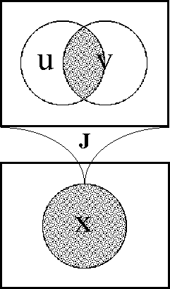
To study the effects of these analytic operators in the simplest possible situation, let us revert to a still more primitive case. Consider the singular proposition J‹u, v› = uv, regarded either as the functional product of the maps u and v or as the logical conjunction of the features u and v, a map whose fiber of truth J–1(1) picks out the single cell of that logical description in the universe of discourse U •. Thus J, or uv, may be treated as a pseudonym for the point whose coordinates are ‹1, 1› in U •.
Analytic Expansion of Conjunction
|
|
In her sufferings she read a great deal and discovered that she had lost something, the possession of which she had previously not been much aware of: a soul.
What is that? It is easily defined negatively: it is simply what curls up and hides when there is any mention of algebraic series.
|
|
| — Robert Musil, The Man Without Qualities, [Mus, 118]
|
Figure 35 pictures the form of conjunction J : B2 → B as a transformation from the 2-dimensional universe [u, v] to the 1-dimensional universe [x]. This is a subtle but significant change of viewpoint on the proposition, attaching an arbitrary but concrete quality to its functional value. Using the language introduced earlier, we can express this change by saying that the proposition J : 〈u, v〉 → B is being recast into the thematized role of a transformation J : [u, v] → [x], where the new variable x takes the part of a thematic variable ¢(J).
Figure 35. Conjunction as Transformation
Tacit Extension of Conjunction
|
|
I teach straying from me, yet who can stray from me?
I follow you whoever you are from the present hour;
My words itch at your ears till you understand them.
|
|
|
— Walt Whitman, Leaves of Grass, [Whi, 83]
|
Earlier I defined the tacit extension operators \(\epsilon\) : X • → Y • as maps embedding each proposition of a given universe X • in a more generously given universe Y • containing X •. Of immediate interest are the tacit extensions \(\epsilon\) : U • → EU •, that locate each proposition of U • in the enlarged context of EU •. In its application to the propositional conjunction J = u v in [u, v], the tacit extension operator \(\epsilon\) produces the proposition \(\epsilon\)J in EU • = [u, v, du, dv]. The extended proposition \(\epsilon\)J may be computed according to the scheme in Table 36, in effect, doing nothing more than conjoining a tautology of [du, dv] to J in U •.
Table 36. Computation of \(\epsilon\)J
| \(\epsilon\)J
|
=
|
J‹u, v›
|
|
|
=
|
u v
|
|
|
=
|
u v (du)(dv) |
+
|
u v (du) dv |
+
|
u v du (dv) |
+
|
u v du dv
|
|
| \(\epsilon\)J
|
=
|
u v (du)(dv)
|
+
|
|
|
|
|
u v (du) dv
|
+
|
|
|
|
|
u v du (dv)
|
+
|
|
|
|
|
u v du dv
|
|
|
|
The lower portion of the Table contains the dispositional features of \(\epsilon\)J arranged in such a way that the variety of ordinary features spreads across the rows and the variety of differential features runs through the columns. This organization serves to facilitate pattern matching in the remainder of our computations. Again, the tacit extension is usually so trivial a concern that we do not always bother to make an explicit note of it, taking it for granted that any function F that is being employed in a differential context is equivalent to \(\epsilon\)F, for a suitable \(\epsilon\).
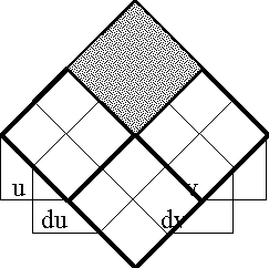
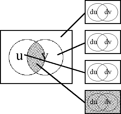
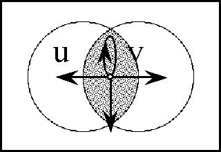
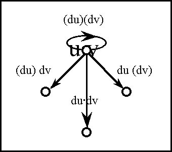
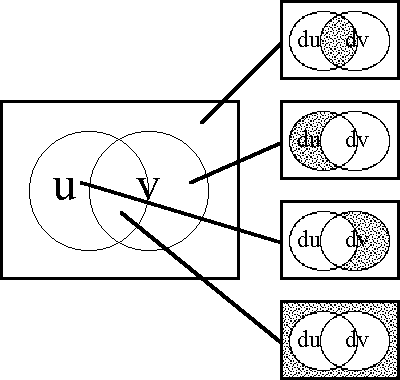
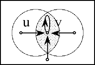
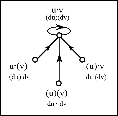
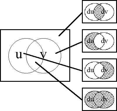
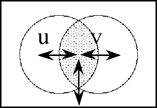
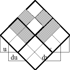
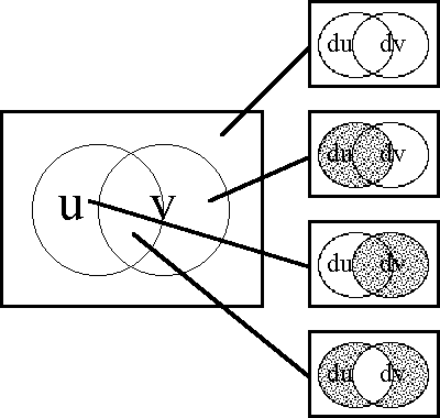
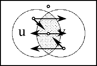
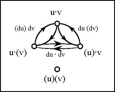
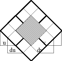
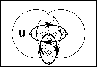
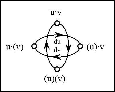
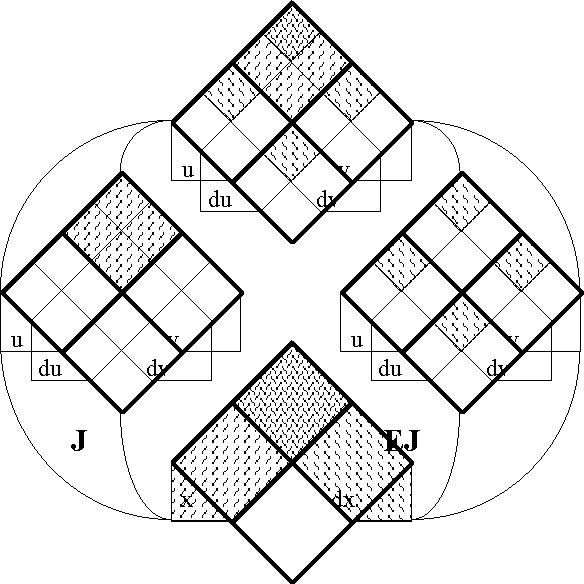
Figures 37-a through 37-d present several pictures of the proposition J and its tacit extension \(\epsilon\)J. Notice in these Figures how \(\epsilon\)J in EU • visibly extends J in U •, by annexing to the indicated cells of J all of the arcs that exit from or flow out of them. In effect, this extension attaches to these cells all of the dispositions that spring from them, in other words, it attributes to these cells all of the conceivable changes that are their issue.
Figure 37-a. Tacit Extension of J (Areal)
Figure 37-b. Tacit Extension of J (Bundle)
Figure 37-c. Tacit Extension of J (Compact)
Figure 37-d. Tacit Extension of J (Digraph)
The computational scheme that was shown in Table 36 treated J as a proposition in U • and formed \(\epsilon\)J as a proposition in EU •. When J is regarded as a mapping J : U • → X • then \(\epsilon\)J must be obtained as a mapping \(\epsilon\)J : EU • → X •. By default, the tacit extension of the map J : [u, v] → [x] is naturally taken to be a particular map, of the following form:
\[\epsilon\]J : [u, v, du, dv] → [x] ⊆ [x, dx]
This is the map that looks like J when painted in the frame of the extended source universe and that takes the same thematic variable in the extended target universe as the one that J already employs.
But the choice of a particular thematic variable, for example x for ¢(J), is a shade more arbitrary than the initial choice of variable names {u, v}. This means that the map I am calling the trope extension, specifically:
\[\eta\]J : [u, v, du, dv] → [dx] ⊆ [x, dx]
since it looks just the same as \(\epsilon\)J in the way that its fibers paint the source domain, belongs just as fully to the family of tacit extensions, generically considered.
These considerations have the practical consequence that all of our computations and illustrations of \(\epsilon\)J perform the double duty of capturing an image of \(\eta\)J as well. In other words, we are saved the work of carrying out calculations and drawing figures for the trope extension \(\eta\)J, because the exercise would be identical to the work already done for \(\epsilon\)J. Since the computations given for \(\epsilon\)J are expressed solely in terms of the variables {u, v, du, dv}, these variables work equally well for finding \(\eta\)J. Furthermore, since each of the above Figures shows only how the level sets of \(\epsilon\)J partition the extended source universe EU • = [u, v, du, dv], all of them serve equally well as portraits of \(\eta\)J.
Enlargement Map of Conjunction
|
|
No one could have established the existence of any details that might not just as well have existed in earlier times too; but all the relations between things had shifted slightly. Ideas that had once been of lean account grew fat.
|
|
| — Robert Musil, The Man Without Qualities, [Mus, 62]
|
The enlargement map EJ is computed from the proposition J by making a particular class of formal substitutions for its variables, in this case u + du for u and v + dv for v, and subsequently expanding the result in whatever way happens to be convenient for the end in view.
Table 38 shows a typical scheme of computation, following a systematic method of exploiting boolean expansions over selected variables, and ultimately developing EJ over the cells of [u, v]. The critical step of this procedure uses the facts that (0, x) = 0 + x = x and (1, x) = 1 + x = (x) for any boolean variable x.
Table 38. Computation of EJ (Method 1)
| EJ
|
=
|
J‹u + du, v + dv›
|
|
|
|
|
|
=
|
(u, du)(v, dv)
|
|
|
|
|
|
=
|
u v J‹1 + du, 1 + dv›
|
+
|
|
|
|
u (v) J‹1 + du, 0 + dv›
|
+
|
|
|
|
(u) v J‹0 + du, 1 + dv›
|
+
|
|
|
|
(u)(v) J‹0 + du, 0 + dv›
|
|
|
|
|
|
=
|
u v J‹(du), (dv)›
|
+
|
|
|
|
u (v) J‹(du), dv ›
|
+
|
|
|
|
(u) v J‹ du , (dv)›
|
+
|
|
|
|
(u)(v) J‹ du , dv ›
|
|
|
| EJ
|
= u v (du)(dv)
|
|
|
|
|
|
|
+ u (v) (du) dv
|
|
|
|
|
|
|
+ (u) v du (dv)
|
|
|
|
|
|
|
+ (u)(v) du dv
|
|
Table 39 exhibits another method that happens to work quickly in this particular case, using distributive laws to multiply things out in an algebraic manner, arranging the notations of feature and fluxion according to a scale of simple character and degree. Proceeding this way leads through an intermediate step which, in chiming the changes of ordinary calculus, should take on a familiar ring. Consequential properties of exclusive disjunction then carry us on to the concluding line.
Table 39. Computation of EJ (Method 2)
| EJ
|
= ‹u + du› \(\cdot\) ‹v + dv›
|
|
|
|
|
|
|
= u v + u dv + v du + du dv
|
|
|
|
|
| EJ
|
= u v (du)(dv)
|
+ u (v) (du) dv
|
+ (u) v du (dv)
|
+ (u)(v) du dv
|
|
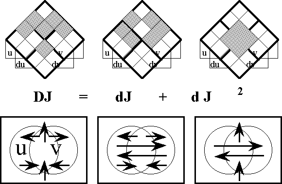
Figures 40-a through 40-d present several views of the enlarged proposition EJ.
Figure 40-a. Enlargement of J (Areal)
Figure 40-b. Enlargement of J (Bundle)
Figure 40-c. Enlargement of J (Compact)
Figure 40-d. Enlargement of J (Digraph)
An intuitive reading of the proposition EJ becomes available at this point, and may be useful. Recall that propositions in the extended universe EU • express the dispositions of system and the constraints that are placed on them. In other words, a differential proposition in EU • can be read as referring to various changes that a system might undergo in and from its various states. In particular, we can understand EJ as a statement that tells us what changes need to be made with regard to each state in the universe of discourse in order to reach the truth of J, that is, the region of the universe where J is true. This interpretation is visibly clear in the Figures above, and appeals to the imagination in a satisfying way, but it has the added benefit of giving fresh meaning to the original name of the shift operator E. Namely, EJ can be read as a proposition that enlarges on the meaning of J, in the sense of explaining its practical bearings and clarifying what it means in terms of the available options for differential action and the consequential effects that result from each choice.
Treated this way, the enlargement EJ has strong ties to the normal use of J, no matter whether it is understood as a proposition or a function, namely, to act as a figurative device for indicating the models of J, in effect, pointing to the interpretive elements in its fiber of truth J–1(1). It is this kind of use that is often compared with the mention of a proposition, and thereby hangs a tale.
Digression : Reflection on Use and Mention
|
|
Reflection is turning a topic over in various aspects and in various lights so that nothing significant about it shall be overlooked — almost as one might turn a stone over to see what its hidden side is like or what is covered by it.
|
|
| — John Dewey, How We Think, [Dew, 57]
|
The contrast drawn in logic between the use and the mention of a proposition corresponds to the difference that we observe in functional terms between using "J " to indicate the region J–1(1) and using "J " to indicate the function J. You may think that one of these uses ought to be proscribed, and logicians are quick to prescribe against their confusion. But there seems to be no likelihood in practice that their interactions can be avoided. If the name "J " is used as a sign of the function J, and if the function J has its use in signifying something else, as would constantly be the case when some future theory of signs has given a functional meaning to every sign whatsoever, then is not "J " by transitivity a sign of the thing itself? There are, of course, two answers to this question. Not every act of signifying or referring need be transitive. Not every warrant or guarantee or certificate is automatically transferable, indeed, not many. Not every feature of a feature is a feature of the featuree. Otherwise we have an inference like the following: If a buffalo is white, and white is a color, then a buffalo is a color. But a buffalo is not, only buff is.
The logical or pragmatic distinction between use and mention is cogent and necessary, and so is the analogous functional distinction between determining a value and determining what determines that value, but so are the normal techniques that we use to make these distinctions apply flexibly in practice. The way that the hue and cry about use and mention is raised in logical discussions, you might be led to think that this single dimension of choices embraces the only kinds of use worth mentioning and the only kinds of mention worth using. It will constitute the expeditionary and taxonomic tasks of that future theory of signs to explore and to classify the many other constellations and dimensions of use and mention that are yet to be opened up by the generative potential of full-fledged sign relations.
|
|
The well-known capacity that thoughts have — as doctors have discovered — for dissolving and dispersing those hard lumps of deep, ingrowing, morbidly entangled conflict that arise out of gloomy regions of the self probably rests on nothing other than their social and worldly nature, which links the individual being with other people and things; but unfortunately what gives them their power of healing seems to be the same as what diminishes the quality of personal experience in them.
|
|
| — Robert Musil, The Man Without Qualities, [Mus, 130]
|
Difference Map of Conjunction
|
|
"It doesn't matter what one does", the Man Without Qualities said to himself, shrugging his shoulders. "In a tangle of forces like this it doesn't make a scrap of difference." He turned away like a man who has learned renunciation, almost indeed like a sick man who shrinks from any intensity of contact. And then, striding through his adjacent dressing-room, he passed a punching-ball that hung there; he gave it a blow far swifter and harder than is usual in moods of resignation or states of weakness.
|
|
| — Robert Musil, The Man Without Qualities, [Mus, 8]
|
With the tacit extension map \(\epsilon\)J and the enlargement map EJ well in place, the difference map DJ can be computed along the lines displayed in Table 41, ending up, in this instance, with an expansion of DJ over the cells of [u, v].
Table 41. Computation of DJ (Method 1)
| DJ
|
=
|
EJ
|
+
|
\(\epsilon\)J
|
|
|
=
|
J‹u + du, v + dv›
|
+
|
J‹u, v›
|
|
|
=
|
(u, du)(v, dv)
|
+
|
u v
|
|
| DJ
|
=
|
0
|
|
|
|
|
|
+
|
u v (du) dv
|
+ u (v)(du) dv
|
|
|
|
|
+
|
u v du (dv)
|
|
+ (u) v du (dv)
|
|
|
|
+
|
u v du dv
|
|
|
+ (u)(v) du dv
|
|
| DJ
|
=
|
u v ((du)(dv))
|
+ u (v)(du) dv
|
+ (u) v du (dv)
|
+ (u)(v) du dv
|
|
Alternatively, the difference map DJ can be expanded over the cells of [du, dv] to arrive at the formulation shown in Table 42. The same development would be obtained from the previous Table by collecting terms in an alternate manner, along the rows rather than the columns of the middle portion of the Table.
Table 42. Computation of DJ (Method 2)
| DJ
|
=
|
\(\epsilon\)J
|
+
|
EJ
|
|
|
=
|
J‹u, v›
|
+
|
J‹u + du, v + dv›
|
|
|
=
|
u v
|
+
|
(u, du)(v, dv)
|
|
|
=
|
0
|
+
|
u dv
|
+
|
v du
|
+
|
du dv
|
| DJ
|
=
|
0
|
+
|
u (du) dv
|
+
|
v du (dv)
|
+
|
((u, v)) du dv
|
|
Even more simply, the same result is reached by matching up the propositional coefficients of \(\epsilon\)J and EJ along the cells of [du, dv] and adding the pairs under boolean sums (that is, "mod 2", where 1 + 1 = 0), as shown in Table 43.
Table 43. Computation of DJ (Method 3)
|
|
| \(\epsilon\)J
|
= u v (du)(dv)
|
+ u v (du) dv
|
+ u v du (dv)
|
+ u v du dv
|
| EJ
|
= u v (du)(dv)
|
+ u (v)(du) dv
|
+ (u) v du (dv)
|
+ (u)(v) du dv
|
|
| DJ
|
= 0 \(\cdot\) (du)(dv)
|
+ u \(\cdot\) (du) dv
|
+ v \(\cdot\) du (dv)
|
+ ((u, v)) du dv
|
|
The difference map DJ can also be given a dispositional interpretation. First, recall that \(\epsilon\)J exhibits the dispositions to change from anywhere in J to anywhere at all, and EJ enumerates the dispositions to change from anywhere at all to anywhere in J. Next, observe that each of these classes of dispositions may be divided in accordance with the case of J versus (J) that applies to their points of departure and destination, as shown below. Then, since the dispositions corresponding to \(\epsilon\)J and EJ have in common the dispositions to preserve J, their symmetric difference (\(\epsilon\)J, EJ) is made up of all the remaining dispositions, which are in fact disposed to cross the boundary of J in one direction or the other. In other words, we may conclude that DJ expresses the collective disposition to make a definite change with respect to J, no matter what value it holds in the current state of affairs.
| \(\epsilon\)J
|
= {Dispositions from J to J }
|
+ {Dispositions from J to (J) }
|
|
|
| EJ
|
= {Dispositions from J to J }
|
+ {Dispositions from (J) to J }
|
|
|
| DJ
|
= (\(\epsilon\)J, EJ)
|
|
|
|
| DJ
|
= {Dispositions from J to (J) }
|
+ {Dispositions from (J) to J }
|
|
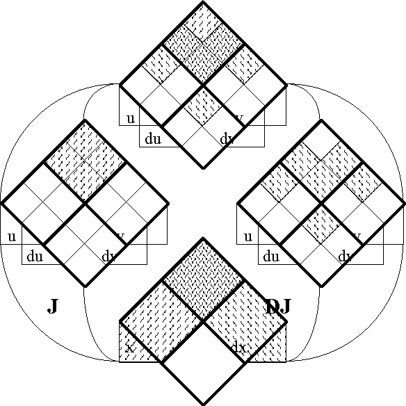
Figures 44-a through 44-d illustrate the difference proposition DJ.
Figure 44-a. Difference Map of J (Areal)
Figure 44-b. Difference Map of J (Bundle)
Figure 44-c. Difference Map of J (Compact)
Figure 44-d. Difference Map of J (Digraph)
Differential of Conjunction
|
|
By deploying discourse throughout a calendar, and by giving a date to each of its elements, one does not obtain a definitive hierarchy of precessions and originalities; this hierarchy is never more than relative to the systems of discourse that it sets out to evaluate.
|
|
| — Michel Foucault, The Archaeology of Knowledge, [Fou, 143]
|
Finally, at long last, the differential proposition dJ can be gleaned from the difference proposition DJ by ranging over the cells of [u, v] and picking out the linear proposition of [du, dv] that is "closest" to the portion of DJ that touches on each point. The idea of distance that would give this definition unequivocal sense has been referred to in cautionary quotes, the kind we use to distance ourselves from taking a final position. There are obvious notions of approximation that suggest themselves, but finding one that can be justified as ultimately correct is not as straightforward as it seems.
|
|
He had drifted into the very heart of the world. From him to the distant beloved was as far as to the next tree.
|
|
| — Robert Musil, The Man Without Qualities, [Mus, 144]
|
Let us venture a guess about where these developments might be heading. From the present vantage point, it appears that the ultimate answer to the quandary of distances and the question of a fitting measure may be that, rather than having the constitution of an analytic series depend on our familiar notions of approach, proximity, and approximation, it will be found preferable, and perhaps unavoidable, to turn the tables and let the orders of approximation be defined in terms of our favored and operative notions of formal analysis. Only the aftermath of this conversion, if it does converge, could be hoped to prove whether this hortatory form of analysis and the cohort idea of an analytic form — the limitary concept of a self-corrective process and the coefficient concept of a completable product — are truly (in practical reality) the more inceptive and persistent of principles and really (for all practical purposes) the more effective and regulative of ideas.
Awaiting that determination, I proceed with what seems like the obvious course, and compute dJ according to the pattern in Table 45.
Table 45. Computation of dJ
| DJ
|
= u v ((du)(dv))
|
+ u (v)(du) dv
|
+ (u) v du (dv)
|
+ (u)(v) du dv
|
| ⇒
|
| dJ
|
= u v (du, dv)
|
+ u (v) dv
|
+ (u) v du
|
+ (u)(v) \(\cdot\) 0
|
|
Figures 46-a through 46-d illustrate the proposition dJ, rounded out in our usual array of prospects. This proposition of EU • is what we refer to as the (first order) differential of J, and normally regard as the differential proposition corresponding to J.
Figure 46-a. Differential of J (Areal)
Figure 46-b. Differential of J (Bundle)
Figure 46-c. Differential of J (Compact)
Figure 46-d. Differential of J (Digraph)
Remainder of Conjunction
|
|
I bequeath myself to the dirt to grow from the grass I love,
If you want me again look for me under your bootsoles.
You will hardly know who I am or what I mean,
But I shall be good health to you nevertheless,
And filter and fibre your blood.
Failing to fetch me at first keep encouraged,
Missing me one place search another,
I stop some where waiting for you
|
|
|
— Walt Whitman, Leaves of Grass, [Whi, 88]
|
Let us now recapitulate the story so far. In effect, we have been carrying out a decomposition of the enlarged proposition EJ in a series of stages. First, we considered the equation EJ = \(\epsilon\)J + DJ, which was involved in the definition of DJ as the difference EJ – \(\epsilon\)J. Next, we contemplated the equation DJ = dJ + rJ, which expresses DJ in terms of two components, the differential dJ that was just extracted and the residual component rJ = DJ – dJ. This remaining proposition rJ can be computed as shown in Table 47.
Table 47. Computation of rJ
|
|
| DJ
|
= u v ((du)(dv))
|
+ u (v)(du) dv
|
+ (u) v du (dv)
|
+ (u)(v) du dv
|
| dJ
|
= u v (du, dv)
|
+ u (v) dv
|
+ (u) v du
|
+ (u)(v) \(\cdot\) 0
|
|
| rJ
|
= u v du dv
|
+ u (v) du dv
|
+ (u) v du dv
|
+ (u)(v) du dv
|
|
As it happens, the remainder rJ falls under the description of a second order differential rJ = d2J. This means that the expansion of EJ in the form:
| EJ
|
=
|
\(\epsilon\)J
|
+
|
DJ
|
|
|
=
|
\(\epsilon\)J
|
+
|
dJ
|
+
|
rJ
|
|
|
=
|
d0J
|
+
|
d1J
|
+
|
d2J
|
which is nothing other than the propositional analogue of a Taylor series, is a decomposition that terminates in a finite number of steps.
Figures 48-a through 48-d illustrate the proposition rJ = d2J, which forms the remainder map of J and also, in this instance, the second order differential of J.
Figure 48-a. Remainder of J (Areal)
Figure 48-b. Remainder of J (Bundle)
Figure 48-c. Remainder of J (Compact)
Figure 48-d. Remainder of J (Digraph)
Summary of Conjunction
To establish a convenient reference point for further discussion, Table 49 summarizes the operator actions that have been computed for the form of conjunction, as exemplified by the proposition J.
Table 49. Computation Summary for J
| \(\epsilon\)J
|
= |
uv |
\(\cdot\) |
1
|
+ |
u(v) |
\(\cdot\) |
0
|
+ |
(u)v |
\(\cdot\) |
0
|
+ |
(u)(v) |
\(\cdot\) |
0
|
| EJ
|
= |
uv |
\(\cdot\) |
(du)(dv)
|
+ |
u(v) |
\(\cdot\) |
(du)dv
|
+ |
(u)v |
\(\cdot\) |
du(dv)
|
+ |
(u)(v) |
\(\cdot\) |
du dv
|
| DJ
|
= |
uv |
\(\cdot\) |
((du)(dv))
|
+ |
u(v) |
\(\cdot\) |
(du)dv
|
+ |
(u)v |
\(\cdot\) |
du(dv)
|
+ |
(u)(v) |
\(\cdot\) |
du dv
|
| dJ
|
= |
uv |
\(\cdot\) |
(du, dv)
|
+ |
u(v) |
\(\cdot\) |
dv
|
+ |
(u)v |
\(\cdot\) |
du
|
+ |
(u)(v) |
\(\cdot\) |
0
|
| rJ
|
= |
uv |
\(\cdot\) |
du dv
|
+ |
u(v) |
\(\cdot\) |
du dv
|
+ |
(u)v |
\(\cdot\) |
du dv
|
+ |
(u)(v) |
\(\cdot\) |
du dv
|
|
Analytic Series : Coordinate Method
|
|
And if he is told that something is the way it is, then he thinks: Well, it could probably just as easily be some other way. So the sense of possibility might be defined outright as the capacity to think how everything could "just as easily" be, and to attach no more importance to what is than to what is not.
|
|
| — Robert Musil, The Man Without Qualities, [Mus, 12]
|
Table 50 exhibits a truth table method for computing the analytic series (or the differential expansion) of a proposition in terms of coordinates.
Table 50. Computation of an Analytic Series in Terms of Coordinates
|
|
|
The first six columns of the Table, taken as a whole, represent the variables of a construct that I describe as the contingent universe [u, v, du, dv, u′, v′ ], or the bundle of contingency spaces [du, dv, u′, v′ ] over the universe [u, v]. Their placement to the left of the double bar indicates that all of them amount to independent variables, but there is a co-dependency among them, as described
by the following equations:
| |
u’ |
= |
u + du |
= |
(u, du) |
|
| |
v’ |
= |
v + du |
= |
(v, dv) |
|
|
These relations correspond to the formal substitutions that are made in defining EJ and DJ. For now, the whole rigamarole of contingency spaces can be regarded as a technical device for achieving the effect of these substitutions, adapted to a setting where functional compositions and other symbolic manipulations are difficult to contemplate and execute.
The five columns to the right of the double bar in Table 50 contain the values of the dependent variables {\(\epsilon\)J, EJ, DJ, dJ, d2J}. These are normally interpreted as values of functions WJ : EU → B or as values of propositions in the extended universe [u, v, du, dv], but the dependencies prevailing in the contingent universe make it possible to regard these same final values as arising via functions on alternative lists of arguments, say, ‹u, v, u′, v′›.
The column for \(\epsilon\)J is computed as J‹u, v› = uv. This, along with the columns for u and v, illustrates the Table's structure-sharing scheme, listing only the initial entries of each constant block.
The column for EJ is computed by means of the following chain of identities, where the contingent variables u′ and v′ are defined as u′ = u + du and v′ = v + dv.
| EJ‹u, v, du, dv›
|
=
|
J‹u + du, v + dv›
|
=
|
J‹u’, v’›
|
|
This makes it easy to determine EJ by inspection, computing the conjunction J‹u′, v′› = u′ v′ from the columns headed u′ and v′. Since all of these forms express the same proposition EJ in EU •, the dependence on du and dv is still present but merely left implicit in the final variant J‹u′, v′›.
- NB. On occasion, it is tempting to use the further notation J′‹u, v› = J‹u′, v′›, especially to suggest a transformation that acts on whole propositions, for example, taking the proposition J into the proposition J′ = EJ. The prime [′] then signifies an action that is mediated by a field of choices, namely, the values that are picked out for the contingent variables in sweeping through the initial universe. But this heaps an unwieldy lot of construed intentions on a rather slight character, and puts too high a premium on the constant correctness of its interpretation. In practice, therefore, it is best to avoid this usage.
Given the values of \(\epsilon\)J and EJ, the columns for the remaining functions can be filled in quickly. The difference map is computed according to the relation DJ = \(\epsilon\)J + EJ. The first order differential dJ is found by looking in each block of constant ‹u, v› and choosing the linear function of ‹du, dv› that best approximates DJ in that block. Finally, the remainder is computed as rJ = DJ + dJ, in this case yielding the second order differential d2J.
Analytic Series : Recap
Let us now summarize the results of Table 50 by writing down for each column, and for each block of constant ‹u, v›, a reasonably canonical symbolic expression for the function of ‹du, dv› that appears there. The synopsis formed in this way is presented in Table 51. As one has a right to expect, it confirms the results that were obtained previously by operating solely in terms of the formal calculus.
Table 51. Computation of an Analytic Series in Symbolic Terms
|
|
|
|
|
|
|
|
|
|
| du dv
|
| du (dv)
|
| (du) dv
|
| (du)(dv)
|
|
| du dv
|
| du (dv)
|
| (du) dv
|
| ((du)(dv))
|
|
|
|
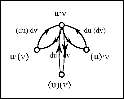
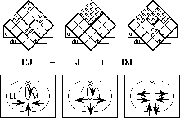
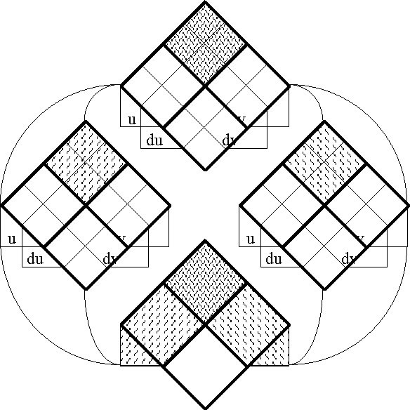
Figures 52 and 53 provide a quick overview of the analysis performed so far, giving the successive decompositions of EJ = J + DJ and DJ = dJ + rJ in two different styles of diagram.
Figure 52. Decomposition of EJ
Figure 53. Decomposition of DJ
Terminological Interlude
|
|
Lastly, my attention was especially attracted, not so much to the scene, as to the mirrors that produced it. These mirrors were broken in parts. Yes, they were marked and scratched; they had been "starred", in spite of their solidity …
|
|
| — Gaston Leroux, The Phantom of the Opera, [Ler, 230]
|
At this point several issues of terminology have accrued enough substance to intrude on our discussion. The remarks of this Section are intended to accomplish two goals. First, I call attention to important aspects of the previous series of Figures, translating into literal terms what they depict in iconic forms, and I restress the most important structural elements that they indicate. Next, I prepare the way for taking on more complex examples of transformations, whose target universes have more than a single dimension.
In talking about the actions of operators it is important to keep in mind the distinctions between the operators per se, their operands, and their results. Furthermore, in working with composite forms of operators W = ‹W1, …, Wn› , transformations F = ‹F1, …, Fn› , and target domains X • = [x1, …, xn], we need to preserve a clear distinction between the compound entity of each given type and any one of its separate components. It is curious, given the usefulness of the concepts operator and operand, that we seem to lack a generic term, formed on the same root, for the corresponding result of an operation. Following the obvious paradigm would lead on to words like opus, opera, and operant, but these words are too affected with clang associations to work well at present, though they might be adapted in time. One current usage gets around this problem by using the substantive map as a systematic epithet to express the result of each operator's action. I am following this practice as far as possible, for example, using the phrase tangent map to denote the end product of the tangent functor acting on its operand map.
- Scholium. See [JGH, 6-9] for a good account of tangent functors and tangent maps in ordinary analysis, and for examples of their use in mechanics. This work as a whole is a model of clarity in applying functorial principles to problems in physical dynamics.
Whenever we focus on isolated propositions, on single components of composite operators, or on the portions of transformations that have 1-dimensional ranges, we are free to shift between the native form of a proposition J : U → B and the thematized form of a mapping J : U • → [x] without much trouble. In these cases we are able to tolerate a higher degree of ambiguity about the precise nature of the input and output domains of an operator than we otherwise might. For example, in the preceding treatment of the example J, and for each operator W in the set {\(\epsilon\), \(\eta\), E, D, d, r}, both the operand J and the result WJ could be viewed in either one of two ways. On the one hand, we could regard them as propositions J : U → B and WJ : EU → B, ignoring the qualitative distinction between the range [x] \(\cong\) B of \(\epsilon\)J and the range [dx] \(\cong\) D of the other types of WJ. This is what we usually do when we content ourselves simply with coloring in regions of venn diagrams. On the other hand, we could view these entities as maps J : U • → [x] = X • and \(\epsilon\)J : EU • → [x] ⊆ EX • or WJ : EU • → [dx] ⊆ EX •, in which case the qualitative characters of the output features are not allowed to go without saying, nor thus at the risk of being forgotten.
At the beginning of this Division I recast the natural form of a proposition J : U → B into the thematic role of a transformation J : U • → [x], where x was a variable recruited to express the newly independent ¢(J). However, in my computations and representations of operator actions I immediately lapsed back to viewing the results as native elements of the extended universe EU •, in other words, as propositions WJ : EU → B, where W ranged over the set {\(\epsilon\), E, D, d, r}. That is as it should be. In fact, I have worked hard to devise a language that gives us all of these competing advantages, the flexibility to exchange terms and types that bear equal information value, and the capacity to reflect as quickly and as wittingly as a controlled reflex on the fibers of our propositions, independently of whether they express amusements, beliefs, or conjectures.
As we take on target spaces of increasing dimension, however, these types of confusions (and confusions of types) become less and less permissible. For this reason, Tables 54 and 55 present a rather detailed summary of the notation and the terminology that I am using here, as applied to the case of J = uv. The rationale of these Tables is not so much to train more elephant guns on this poor drosophila of an example, but to establish the general paradigm with enough solidity to bear the weight of abstraction that is coming on down the road.
Table 54 provides basic notation and descriptive information for the objects and operators that are used used in this Example, giving the generic type (or broadest defined type) for each entity. Here, the operators W in {e, E, D, d, r} and their components W in {\(\epsilon\), \(\eta\), E, D, d, r} both have the same broad type W, W : (U • → X •) → (EU • → EX •), as would be expected of operators that map transformations J : U • → X • to extended transformations WJ, WJ : EU • → EX •.
Table 54. Cast of Characters: Expansive Subtypes of Objects and Operators
| Item
|
Notation
|
Description
|
Type
|
| U •
|
= [u, v]
|
Source Universe
|
[B2]
|
| X •
|
= [x]
|
Target Universe
|
[B1]
|
| EU •
|
= [u, v, du, dv]
|
Extended Source Universe
|
[B2 × D2]
|
| EX •
|
= [x, dx]
|
Extended Target Universe
|
[B1 × D1]
|
| J
|
J : U → B
|
Proposition
|
(B2 → B) ∈ [B2]
|
| J
|
J : U • → X •
|
Transformation, or Mapping
|
[B2] → [B1]
|
|
|
| W :
|
| U • → EU • ,
|
| X • → EX • ,
|
| (U • → X •)
|
| →
|
| (EU • → EX •) ,
|
| for each W in the set:
|
| {\(\epsilon\), \(\eta\), E, D, d}
|
|
|
|
|
| [B2] → [B2 × D2] ,
|
| [B1] → [B1 × D1] ,
|
| ([B2] → [B1])
|
| →
|
| ([B2 × D2] → [B1 × D1])
|
|
|
|
|
|
| \(\epsilon\)
|
| \(\eta\)
|
| E
|
| D
|
| d
|
|
|
| Tacit Extension Operator |
\(\epsilon\)
|
| Trope Extension Operator |
\(\eta\)
|
| Enlargement Operator |
E
|
| Difference Operator |
D
|
| Differential Operator |
d
|
|
|
|
| W :
|
| U • → TU • = EU • ,
|
| X • → TX • = EX • ,
|
| (U • → X •)
|
| →
|
| (TU • → TX •) ,
|
| for each W in the set:
|
| {e, E, D, T}
|
|
|
|
|
| [B2] → [B2 × D2] ,
|
| [B1] → [B1 × D1] ,
|
| ([B2] → [B1])
|
| →
|
| ([B2 × D2] → [B1 × D1])
|
|
|
|
|
|
|
|
|
| Radius Operator |
e = ‹\(\epsilon\), \(\eta\)›
|
| Secant Operator |
E = ‹\(\epsilon\), E›
|
| Chord Operator |
D = ‹\(\epsilon\), D›
|
| Tangent Functor |
T = ‹\(\epsilon\), d›
|
|
Table 55 supplies a more detailed outline of terminology for operators and their results. Here, I list the restrictive subtype (or narrowest defined subtype) that applies to each entity, and I indicate across the span of the Table the whole spectrum of alternative types that color the interpretation of each symbol. Accordingly, each of the component operator maps WJ, since their ranges are 1-dimensional (of type B1 or D1), can be regarded either as propositions WJ : EU → B or as logical transformations WJ : EU • → X •. As a rule, the plan of the Table allows us to name each entry by detaching the adjective at the left of its row and prefixing it to the generic noun at the top of its column. In one case, however, it is customary to depart from this scheme. Because the phrase differential proposition, applied to the result dJ : EU → D, does not distinguish it from the general run of differential propositions G : EU → B, it is usual to single out dJ as the tangent proposition of J.
Table 55. Synopsis of Terminology: Restrictive and Alternative Subtypes
|
|
Operator
|
Proposition
|
Map
|
|
|
| \(\epsilon\) :
|
| U • → EU • , X • → EX • ,
|
| (U • → X •) → (EU • → X •)
|
|
| \(\epsilon\)J :
|
| 〈u, v, du, dv〉 → B
|
| B2 × D2 → B
|
|
| \(\epsilon\)J :
|
| [u, v, du, dv] → [x]
|
| [B2 × D2] → [B1]
|
|
|
|
| \(\eta\) :
|
| U • → EU • , X • → EX • ,
|
| (U • → X •) → (EU • → dX •)
|
|
| \(\eta\)J :
|
| 〈u, v, du, dv〉 → D
|
| B2 × D2 → D
|
|
| \(\eta\)J :
|
| [u, v, du, dv] → [dx]
|
| [B2 × D2] → [D1]
|
|
|
|
| E :
|
| U • → EU • , X • → EX • ,
|
| (U • → X •) → (EU • → dX •)
|
|
| EJ :
|
| 〈u, v, du, dv〉 → D
|
| B2 × D2 → D
|
|
| EJ :
|
| [u, v, du, dv] → [dx]
|
| [B2 × D2] → [D1]
|
|
|
|
| D :
|
| U • → EU • , X • → EX • ,
|
| (U • → X •) → (EU • → dX •)
|
|
| DJ :
|
| 〈u, v, du, dv〉 → D
|
| B2 × D2 → D
|
|
| DJ :
|
| [u, v, du, dv] → [dx]
|
| [B2 × D2] → [D1]
|
|
|
|
| d :
|
| U • → EU • , X • → EX • ,
|
| (U • → X •) → (EU • → dX •)
|
|
| dJ :
|
| 〈u, v, du, dv〉 → D
|
| B2 × D2 → D
|
|
| dJ :
|
| [u, v, du, dv] → [dx]
|
| [B2 × D2] → [D1]
|
|
|
|
| r :
|
| U • → EU • , X • → EX • ,
|
| (U • → X •) → (EU • → dX •)
|
|
| rJ :
|
| 〈u, v, du, dv〉 → D
|
| B2 × D2 → D
|
|
| rJ :
|
| [u, v, du, dv] → [dx]
|
| [B2 × D2] → [D1]
|
|
|
|
| e = ‹\(\epsilon\), \(\eta\)› :
|
| U • → EU • , X • → EX • ,
|
| (U • → X •) → (EU • → EX •)
|
|
|
| eJ :
|
| [u, v, du, dv] → [x, dx]
|
| [B2 × D2] → [B × D]
|
|
|
|
| E = ‹\(\epsilon\), E› :
|
| U • → EU • , X • → EX • ,
|
| (U • → X •) → (EU • → EX •)
|
|
|
| EJ :
|
| [u, v, du, dv] → [x, dx]
|
| [B2 × D2] → [B × D]
|
|
|
|
| D = ‹\(\epsilon\), D› :
|
| U • → EU • , X • → EX • ,
|
| (U • → X •) → (EU • → EX •)
|
|
|
| DJ :
|
| [u, v, du, dv] → [x, dx]
|
| [B2 × D2] → [B × D]
|
|
|
|
| T = ‹\(\epsilon\), d› :
|
| U • → EU • , X • → EX • ,
|
| (U • → X •) → (EU • → EX •)
|
|
| dJ :
|
| 〈u, v, du, dv〉 → D
|
| B2 × D2 → D
|
|
| TJ :
|
| [u, v, du, dv] → [x, dx]
|
| [B2 × D2] → [B × D]
|
|
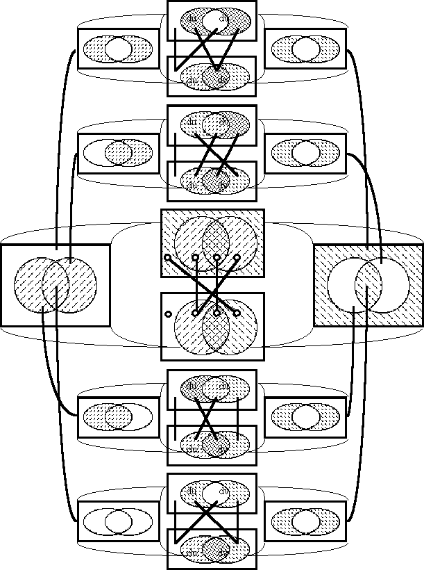
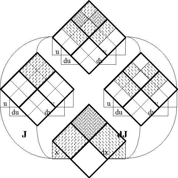
End of Perfunctory Chatter : Time to Roll the Clip!
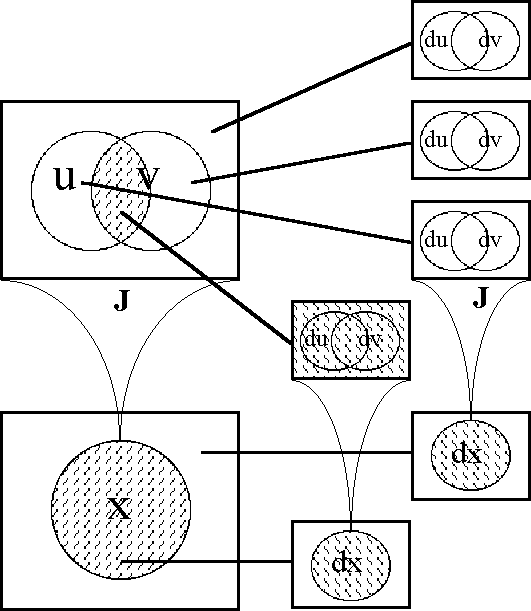
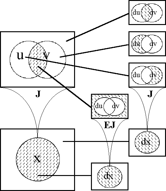
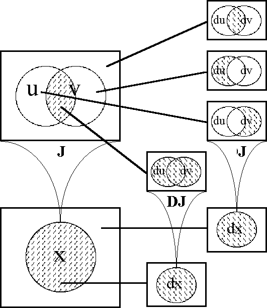
Two steps remain to finish the analysis of J that I began so long ago. First, I need to paste the accumulated heap of flat pictures into the frames of transformations, filling out the shapes of the operator maps WJ : EU • → EX •. This scheme is executed in two styles, using the areal views in Figures 56-a and the box views in Figures 56-b. Finally, in Figures 57-1 to 57-4 I put all the pieces together to construct the full operator diagrams for W : J → WJ. There is a large amount of redundancy in these three series of figures. At this early stage of exposition I thought that it would be better not to tax the reader's imagination, and to guarantee that the author, at least, has worked through the relevant exercises. I hope the reader will excuse the flagrant use of space and try to view these snapshots as successive frames in the animation of logic that they are meant to become.
Operator Maps : Areal Views
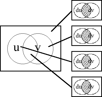
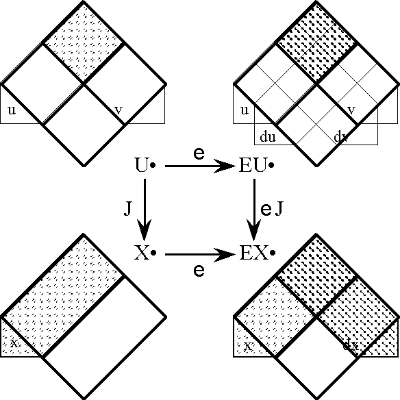
Figure 56-a1. Radius Map of the Conjunction J = uv
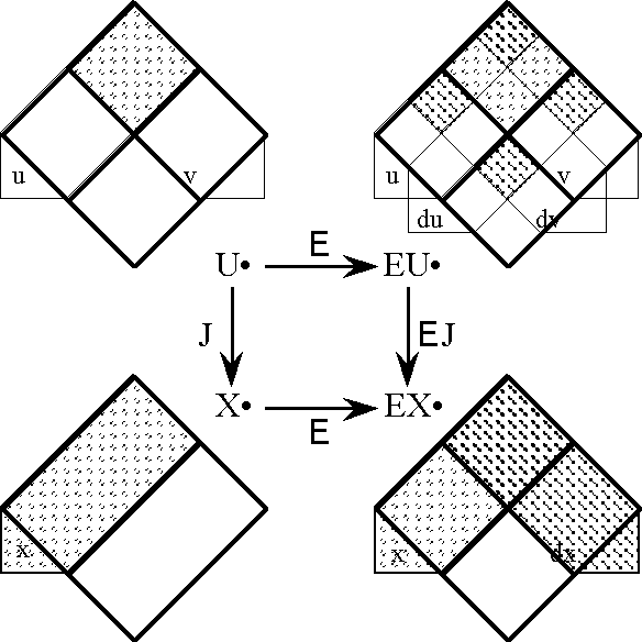
Figure 56-a2. Secant Map of the Conjunction J = uv
Figure 56-a3. Chord Map of the Conjunction J = uv
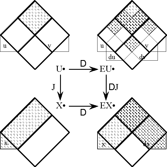
Figure 56-a4. Tangent Map of the Conjunction J = uv
Operator Maps : Box Views
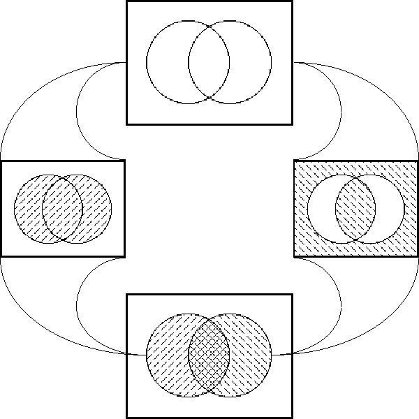
Figure 56-b1. Radius Map of the Conjunction J = uv
Figure 56-b2. Secant Map of the Conjunction J = uv
Figure 56-b3. Chord Map of the Conjunction J = uv
Figure 56-b4. Tangent Map of the Conjunction J = uv
Operator Diagrams for the Conjunction J = uv
Figure 57-1. Radius Operator Diagram for the Conjunction J = uv
Figure 57-2. Secant Operator Diagram for the Conjunction J = uv
Figure 57-3. Chord Operator Diagram for the Conjunction J = uv
Figure 57-4. Tangent Functor Diagram for the Conjunction J = uv
Taking Aim at Higher Dimensional Targets
|
|
The past and present wilt . . . . I have filled them and
emptied them,
And proceed to fill my next fold of the future.
|
|
|
— Walt Whitman, Leaves of Grass, [Whi, 87]
|
In the next Subdivision I consider a logical transformation F that has the concrete type F : [u, v] → [x, y] and the abstract type F : [B2] → [B2]. From the standpoint of propositional calculus, the task of understanding such a transformation is naturally approached by parsing it into component maps with 1-dimensional ranges, as follows:
| F
|
=
|
‹f, g›
|
=
|
‹F1, F2›
|
:
|
[u, v]
|
→
|
[x, y]
|
| where
|
f
|
=
|
F1
|
:
|
[u, v]
|
→
|
[x]
|
| and
|
g
|
=
|
F2
|
:
|
[u, v]
|
→
|
[y]
|
|
Then one tackles the separate components, now viewed as propositions Fi : U → B, one at a time. At the completion of this analytic phase, one returns to the task of synthesizing all of these partial and transient impressions into an agile form of integrity, a solidly coordinated and deeply integrated comprehension of the ongoing transformation. (Very often, of course, in tangling with refractory cases, one never gets as far as the beginning again.)
Let us now refer to the dimension of the target space or codomain as the toll (or tole) of a transformation, as distinguished from the dimension of the range or image that is customarily called the rank. When we keep to transformations with a toll of 1, as J : [u, v] → [x], we tend to get lazy about distinguishing a logical transformation from its component propositions. However, if we deal with transformations of a higher toll, this form of indolence can no longer be tolerated.
Well, perhaps we can carry it a little further. After all, the operator result WJ : EU • → EX • is a map of toll 2, and cannot be unfolded in one piece as a proposition. But when a map has rank 1, like \(\epsilon\)J : EU → X ⊆ EX or dJ : EU → dX ⊆ EX, we naturally choose to concentrate on the 1-dimensional range of the operator result WJ, ignoring the final difference in quality between the spaces X and dX, and view WJ as a proposition about EU.
In this way, an initial ambivalence about the role of the operand J conveys a double duty to the result WJ. The pivot that is formed by our focus of attention is essential to the linkage that transfers this double moment, as the whole process takes its bearing and wheels around the precise measure of a narrow bead that we can draw on the range of WJ. This is the escapement that it takes to get away with what may otherwise seem to be a simple duplicity, and this is the tolerance that is needed to counterbalance a certain arrogance of equivocation, by all of which machinations we make ourselves free to indicate the operator results WJ as propositions or as transformations, indifferently.
But that's it, and no further. Neglect of these distinctions in range and target universes of higher dimensions is bound to cause a hopeless confusion. To guard against these adverse prospects, Tables 58 and 59 lay the groundwork for discussing a typical map F : [B2] → [B2], and begin to pave the way, to some extent, for discussing any transformation of the form F : [Bn] → [Bk].
Table 58. Cast of Characters: Expansive Subtypes of Objects and Operators
| Item
|
Notation
|
Description
|
Type
|
| U •
|
= [u, v]
|
Source Universe
|
[Bn]
|
| X •
|
|
Target Universe
|
[Bk]
|
| EU •
|
= [u, v, du, dv]
|
Extended Source Universe
|
[Bn × Dn]
|
| EX •
|
| = [x, y, dx, dy]
|
| = [f, g, df, dg]
|
|
Extended Target Universe
|
[Bk × Dk]
|
| F
|
F = ‹f, g› : U • → X •
|
Transformation, or Mapping
|
[Bn] → [Bk]
|
|
|
| f, g : U → B
|
| f : U → [x] ⊆ X •
|
| g : U → [y] ⊆ X •
|
|
|
| Bn → B
|
| ∈ (Bn, Bn → B)
|
| = (Bn +→ B) = [Bn]
|
|
|
|
| W :
|
| U • → EU • ,
|
| X • → EX • ,
|
| (U • → X •)
|
| →
|
| (EU • → EX •) ,
|
| for each W in the set:
|
| {\(\epsilon\), \(\eta\), E, D, d}
|
|
|
|
|
| [Bn] → [Bn × Dn] ,
|
| [Bk] → [Bk × Dk] ,
|
| ([Bn] → [Bk])
|
| →
|
| ([Bn × Dn] → [Bk × Dk])
|
|
|
|
|
|
| \(\epsilon\)
|
| \(\eta\)
|
| E
|
| D
|
| d
|
|
|
| Tacit Extension Operator |
\(\epsilon\)
|
| Trope Extension Operator |
\(\eta\)
|
| Enlargement Operator |
E
|
| Difference Operator |
D
|
| Differential Operator |
d
|
|
|
|
| W :
|
| U • → TU • = EU • ,
|
| X • → TX • = EX • ,
|
| (U • → X •)
|
| →
|
| (TU • → TX •) ,
|
| for each W in the set:
|
| {e, E, D, T}
|
|
|
|
|
| [Bn] → [Bn × Dn] ,
|
| [Bk] → [Bk × Dk] ,
|
| ([Bn] → [Bk])
|
| →
|
| ([Bn × Dn] → [Bk × Dk])
|
|
|
|
|
|
|
|
|
| Radius Operator |
e = ‹\(\epsilon\), \(\eta\)›
|
| Secant Operator |
E = ‹\(\epsilon\), E›
|
| Chord Operator |
D = ‹\(\epsilon\), D›
|
| Tangent Functor |
T = ‹\(\epsilon\), d›
|
|
Table 59. Synopsis of Terminology: Restrictive and Alternative Subtypes
|
|
Operator
or
Operand
|
Proposition
or
Component
|
Transformation
or
Mapping
|
| Operand
|
| F = ‹F1, F2›
|
| F = ‹f, g› : U → X
|
|
| Fi : 〈u, v〉 → B
|
| Fi : Bn → B
|
|
| F : [u, v] → [x, y]
|
| F : Bn → Bk
|
|
|
|
| \(\epsilon\) :
|
| U • → EU • , X • → EX • ,
|
| (U • → X •) → (EU • → X •)
|
|
| \(\epsilon\)Fi :
|
| 〈u, v, du, dv〉 → B
|
| Bn × Dn → B
|
|
| \(\epsilon\)F :
|
| [u, v, du, dv] → [x, y]
|
| [Bn × Dn] → [Bk]
|
|
|
|
| \(\eta\) :
|
| U • → EU • , X • → EX • ,
|
| (U • → X •) → (EU • → dX •)
|
|
| \(\eta\)Fi :
|
| 〈u, v, du, dv〉 → D
|
| Bn × Dn → D
|
|
| \(\eta\)F :
|
| [u, v, du, dv] → [dx, dy]
|
| [Bn × Dn] → [Dk]
|
|
|
|
| E :
|
| U • → EU • , X • → EX • ,
|
| (U • → X •) → (EU • → dX •)
|
|
| EFi :
|
| 〈u, v, du, dv〉 → D
|
| Bn × Dn → D
|
|
| EF :
|
| [u, v, du, dv] → [dx, dy]
|
| [Bn × Dn] → [Dk]
|
|
|
|
| D :
|
| U • → EU • , X • → EX • ,
|
| (U • → X •) → (EU • → dX •)
|
|
| DFi :
|
| 〈u, v, du, dv〉 → D
|
| Bn × Dn → D
|
|
| DF :
|
| [u, v, du, dv] → [dx, dy]
|
| [Bn × Dn] → [Dk]
|
|
|
|
| d :
|
| U • → EU • , X • → EX • ,
|
| (U • → X •) → (EU • → dX •)
|
|
| dFi :
|
| 〈u, v, du, dv〉 → D
|
| Bn × Dn → D
|
|
| dF :
|
| [u, v, du, dv] → [dx, dy]
|
| [Bn × Dn] → [Dk]
|
|
|
|
| r :
|
| U • → EU • , X • → EX • ,
|
| (U • → X •) → (EU • → dX •)
|
|
| rFi :
|
| 〈u, v, du, dv〉 → D
|
| Bn × Dn → D
|
|
| rF :
|
| [u, v, du, dv] → [dx, dy]
|
| [Bn × Dn] → [Dk]
|
|
|
|
| e = ‹\(\epsilon\), \(\eta\)› :
|
| U • → EU • , X • → EX • ,
|
| (U • → X •) → (EU • → EX •)
|
|
|
| eF :
|
| [u, v, du, dv] → [x, y, dx, dy]
|
| [Bn × Dn] → [Bk × Dk]
|
|
|
|
| E = ‹\(\epsilon\), E› :
|
| U • → EU • , X • → EX • ,
|
| (U • → X •) → (EU • → EX •)
|
|
|
| EF :
|
| [u, v, du, dv] → [x, y, dx, dy]
|
| [Bn × Dn] → [Bk × Dk]
|
|
|
|
| D = ‹\(\epsilon\), D› :
|
| U • → EU • , X • → EX • ,
|
| (U • → X •) → (EU • → EX •)
|
|
|
| DF :
|
| [u, v, du, dv] → [x, y, dx, dy]
|
| [Bn × Dn] → [Bk × Dk]
|
|
|
|
| T = ‹\(\epsilon\), d› :
|
| U • → EU • , X • → EX • ,
|
| (U • → X •) → (EU • → EX •)
|
|
| dFi :
|
| 〈u, v, du, dv〉 → D
|
| Bn × Dn → D
|
|
| TF :
|
| [u, v, du, dv] → [x, y, dx, dy]
|
| [Bn × Dn] → [Bk × Dk]
|
|
Transformations of Type B2 → B2
To take up a slightly more complex example, but one that remains simple enough to pursue through a complete series of developments, consider the transformation from U • = [u, v] to X • = [x, y] that is defined by the following system of equations:
|
|
x
|
=
|
f‹u, v›
|
=
|
((u)(v))
|
|
|
|
y
|
=
|
g‹u, v›
|
=
|
((u, v))
|
|
|
The component notation F = ‹F1, F2› = ‹f, g› : U • → X • allows us to give a name and a type to this transformation, and permits us to define it by means of the compact description that follows:
|
|
‹x, y›
|
=
|
F‹u, v›
|
=
|
‹((u)(v)), ((u, v))›
|
|
|
The information that defines the logical transformation F can be represented in the form of a truth table, as in Table 60. To cut down on subscripts in this example I continue to use plain letter equivalents for all components of spaces and maps.
Table 60. Propositional Transformation
| u
|
v
|
f
|
g
|
|
|
|
|
|
|
|
|
((u)(v))
|
((u, v))
|
Figure 61 shows how one might paint a picture of the logical transformation F on the canvass that was earlier primed for this purpose (way back in Figure 30).
Figure 61. Propositional Transformation
Figure 62 extracts the gist of Figure 61, exemplifying a style of diagram that is adequate for most purposes.
Figure 62. Propositional Transformation (Short Form)
Figure 63 give a more complete picture of the transformation F, showing how the points of U • are transformed into points of X •. The lines that cross from one universe to the other trace the action that F induces on points, in other words, they depict the aspect of the transformation that acts as a mapping from points to points, and chart its effects on the elements that are variously called cells, points, positions, or singular propositions.
Figure 63. Transformation of Positions
Table 64 shows how the action of the transformation F on cells or points is computed in terms of coordinates.
Table 64. Transformation of Positions
| u v
|
x
|
y
|
x y
|
x (y)
|
(x) y
|
(x)(y)
|
X • = [x, y ]
|
|
|
|
|
|
|
|
|
|
|
|
((u)(v))
|
((u, v))
|
u v
|
(u, v)
|
(u)(v)
|
( )
|
U • = [u, v ]
|
Table 65 extends this scheme from single cells to arbitrary regions of the source and target universes, and illustrates a form of computation that can be used to determine how a logical transformation acts on all of the propositions in the universe. The way that a transformation of positions affects the propositions, or any other structure that can be built on top of the positions, is normally called the induced action of the given transformation on the system of structures in question.
Table 65. Induced Transformation on Propositions
| X •
|
|
U •
|
| fi‹x, y›
|
|
|
|
fj‹u, v›
|
|
|
|
|
|
|
| ()
|
| (x)(y)
|
| (x) y
|
| (x)
|
| x (y)
|
| (y)
|
| (x, y)
|
| (x y)
|
|
| 0 0 0 0
|
| 0 0 0 1
|
| 0 0 1 0
|
| 0 0 1 1
|
| 0 1 0 0
|
| 0 1 0 1
|
| 0 1 1 0
|
| 0 1 1 1
|
|
| ()
|
| ()
|
| (u)(v)
|
| (u)(v)
|
| (u, v)
|
| (u, v)
|
| (u v)
|
| (u v)
|
|
|
| f8
|
| f9
|
| f10
|
| f11
|
| f12
|
| f13
|
| f14
|
| f15
|
|
| x y
|
| ((x, y))
|
| y
|
| (x (y))
|
| x
|
| ((x) y)
|
| ((x)(y))
|
| (())
|
|
| 1 0 0 0
|
| 1 0 0 1
|
| 1 0 1 0
|
| 1 0 1 1
|
| 1 1 0 0
|
| 1 1 0 1
|
| 1 1 1 0
|
| 1 1 1 1
|
|
| u v
|
| u v
|
| ((u, v))
|
| ((u, v))
|
| ((u)(v))
|
| ((u)(v))
|
| (())
|
| (())
|
|
| f8
|
| f8
|
| f9
|
| f9
|
| f14
|
| f14
|
| f15
|
| f15
|
|
Given the alphabets U = {u, v} and X = {x, y}, along with the corresponding universes of discourse U • and X • \(\cong\) [B2], how many logical transformations of the general form G = ‹G1, G2› : U • → X • are there?
Since G1 and G2 can be any propositions of the type B2 → B, there are 24 = 16 choices for each of the maps G1 and G2, and thus there are 24\(\cdot\)24 = 28 = 256 different mappings altogether of the form G : U • → X •. The set of all functions of a given type is customarily denoted by placing its type indicator in parentheses, in the present instance writing (U • → X •) = {G : U • → X •}, and so the cardinality of this function space can be most conveniently summed up by writing |(U • → X •)| = |(B2 → B2)| = 44 = 256.
Given any transformation G = ‹G1, G2› : U • → X • of this type, one can define a couple of further transformations, related to G, that operate between the extended universes, EU • and EX •, of its source and target domains.
First, the enlargement map (or the secant transformation) EG = ‹EG1, EG2› : EU • → EX • is defined by the following set of component equations:
Second, the difference map (or the chordal transformation) DG = ‹DG1, DG2› : EU • → EX • is defined in component-wise fashion as the boolean sum of the initial proposition Gi and the enlarged proposition EGi, for i = 1, 2, according to the following set of equations:
| DGi
|
=
|
Gi‹u, v›
|
+
|
EGi‹u, v, du, dv›
|
|
|
=
|
Gi‹u, v›
|
+
|
Gi‹u + du, v + dv›
|
|
Maintaining a strict analogy with ordinary difference calculus would perhaps have us write DGi = EGi – Gi, but the sum and difference operations are the same thing in boolean arithmetic. It is more often natural in the logical context to consider an initial proposition q, then to compute the enlargement Eq, and finally to determine the difference Dq = q + Eq, so we let the variant order of terms reflect this sequence of considerations.
Viewed in this light the difference operator D is imagined to be a function of very wide scope and polymorphic application, one that is able to realize the association between each transformation G and its difference map DG, for instance, taking the function space (U • → X •) into (EU • → EX •). Given the interpretive flexibility of contexts in which we are allowing a proposition to appear, it should be clear that an operator of this scope is not at all a trivial matter to define properly, and may take some trouble to work out. For the moment, let's content ourselves with returning to particular cases.
In their application to the present example, namely, the logical transformation F = ‹f, g› = ‹((u)(v)), ((u, v))›, the operators E and D respectively produce the enlarged map EF = ‹Ef, Eg› and the difference map DF = ‹Df, Dg›, whose components can be given as follows, if the reader, in lieu of a special font for the logical parentheses, can forgive a syntactically bilingual formulation:
| Ef
|
=
|
((u + du)(v + dv))
|
| Eg
|
=
|
((u + du, v + dv))
|
|
| Df
|
=
|
((u)(v))
|
+
|
((u + du)(v + dv))
|
| Dg
|
=
|
((u, v))
|
+
|
((u + du, v + dv))
|
|
But these initial formulas are purely definitional, and help us little in understanding either the purpose of the operators or the meaning of their results. Working symbolically, let us apply the same method to the separate components f and g that we earlier used on J. This work is recorded in Appendix 1 and a summary of the results is presented in Tables 66-i and 66-ii.
Table 66-i. Computation Summary for f‹u, v› = ((u)(v))
| \(\epsilon\)f
|
= |
uv |
\(\cdot\) |
1
|
+ |
u(v) |
\(\cdot\) |
1
|
+ |
(u)v |
\(\cdot\) |
1
|
+ |
(u)(v) |
\(\cdot\) |
0
|
| Ef
|
= |
uv |
\(\cdot\) |
(du dv)
|
+ |
u(v) |
\(\cdot\) |
(du (dv))
|
+ |
(u)v |
\(\cdot\) |
((du) dv)
|
+ |
(u)(v) |
\(\cdot\) |
((du)(dv))
|
| Df
|
= |
uv |
\(\cdot\) |
du dv
|
+ |
u(v) |
\(\cdot\) |
du (dv)
|
+ |
(u)v |
\(\cdot\) |
(du) dv
|
+ |
(u)(v) |
\(\cdot\) |
((du)(dv))
|
| df
|
= |
uv |
\(\cdot\) |
0
|
+ |
u(v) |
\(\cdot\) |
du
|
+ |
(u)v |
\(\cdot\) |
dv
|
+ |
(u)(v) |
\(\cdot\) |
(du, dv)
|
| rf
|
= |
uv |
\(\cdot\) |
du dv
|
+ |
u(v) |
\(\cdot\) |
du dv
|
+ |
(u)v |
\(\cdot\) |
du dv
|
+ |
(u)(v) |
\(\cdot\) |
du dv
|
|
Table 66-ii. Computation Summary for g‹u, v› = ((u, v))
| \(\epsilon\)g
|
= |
uv |
\(\cdot\) |
1
|
+ |
u(v) |
\(\cdot\) |
0
|
+ |
(u)v |
\(\cdot\) |
0
|
+ |
(u)(v) |
\(\cdot\) |
1
|
| Eg
|
= |
uv |
\(\cdot\) |
((du, dv))
|
+ |
u(v) |
\(\cdot\) |
(du, dv)
|
+ |
(u)v |
\(\cdot\) |
(du, dv)
|
+ |
(u)(v) |
\(\cdot\) |
((du, dv))
|
| Dg
|
= |
uv |
\(\cdot\) |
(du, dv)
|
+ |
u(v) |
\(\cdot\) |
(du, dv)
|
+ |
(u)v |
\(\cdot\) |
(du, dv)
|
+ |
(u)(v) |
\(\cdot\) |
(du, dv)
|
| dg
|
= |
uv |
\(\cdot\) |
(du, dv)
|
+ |
u(v) |
\(\cdot\) |
(du, dv)
|
+ |
(u)v |
\(\cdot\) |
(du, dv)
|
+ |
(u)(v) |
\(\cdot\) |
(du, dv)
|
| rg
|
= |
uv |
\(\cdot\) |
0
|
+ |
u(v) |
\(\cdot\) |
0
|
+ |
(u)v |
\(\cdot\) |
0
|
+ |
(u)(v) |
\(\cdot\) |
0
|
|
Table 67 shows how to compute the analytic series for F = ‹f, g› = ‹((u)(v)), ((u, v))› in terms of coordinates, and Table 68 recaps these results in symbolic terms, agreeing with earlier derivations.
Table 67. Computation of an Analytic Series in Terms of Coordinates
|
|
| \(\epsilon\)f
|
\(\epsilon\)g
|
|
|
|
|
|
|
|
|
|
|
|
|
|
|
|
|
|
|
|
|
|
|
|
|
|
|
|
|
|
|
Table 68. Computation of an Analytic Series in Symbolic Terms
| u v
|
f g
|
Df
|
Dg
|
df
|
dg
|
d2f
|
d2g
|
|
|
|
| ((du)(dv))
|
| (du) dv
|
| du (dv)
|
| du dv
|
|
| (du, dv)
|
| (du, dv)
|
| (du, dv)
|
| (du, dv)
|
|
|
| (du, dv)
|
| (du, dv)
|
| (du, dv)
|
| (du, dv)
|
|
|
|
Figure 69 gives a graphical picture of the difference map DF = ‹Df, Dg› for the transformation F = ‹f, g› = ‹((u)(v)), ((u, v))›. This depicts the same information about Df and Dg that was given in the corresponding rows of the computation summary in Tables 66-i and 66-ii, excerpted here:
|
|
| Df
|
= |
uv |
\(\cdot\) |
du dv
|
+ |
u(v) |
\(\cdot\) |
du (dv)
|
+ |
(u)v |
\(\cdot\) |
(du) dv
|
+ |
(u)(v) |
\(\cdot\) |
((du)(dv))
|
|
|
| Dg
|
= |
uv |
\(\cdot\) |
(du, dv)
|
+ |
u(v) |
\(\cdot\) |
(du, dv)
|
+ |
(u)v |
\(\cdot\) |
(du, dv)
|
+ |
(u)(v) |
\(\cdot\) |
(du, dv)
|
|
|
|
Figure 69. Difference Map of F = ‹f, g› = ‹((u)(v)), ((u, v))›
Figure 70-a shows a graphical way of picturing the tangent functor map dF = ‹df, dg› for the transformation F = ‹f, g› = ›((u)(v)), ((u, v))›. This amounts to the same information about df and dg that was given in the computation summary of Tables 66-i and 66-ii, the relevant rows of which are repeated here:
|
|
| df
|
= |
uv |
\(\cdot\) |
0
|
+ |
u(v) |
\(\cdot\) |
du
|
+ |
(u)v |
\(\cdot\) |
dv
|
+ |
(u)(v) |
\(\cdot\) |
(du, dv)
|
|
|
| dg
|
= |
uv |
\(\cdot\) |
(du, dv)
|
+ |
u(v) |
\(\cdot\) |
(du, dv)
|
+ |
(u)v |
\(\cdot\) |
(du, dv)
|
+ |
(u)(v) |
\(\cdot\) |
(du, dv)
|
|
|
|
Figure 70-a. Tangent Functor Diagram for F‹u, v› = ‹((u)(v)), ((u, v))›
Figure 70-b shows another way to picture the action of the tangent functor on the logical transformation F‹u, v› = ‹((u)(v)), ((u, v))›, roughly in the style of the bundle of universes type of diagram.
 Figure 70-b. Tangent Functor Ferris Wheel for F‹u, v› = ‹((u)(v)), ((u, v))› - Nota Bene. The original Figure 70-b lost some of its labeling in a succession of platform metamorphoses over the years, so I have included an Ascii version below to indicate where the missing labels go.
o-----------------------o o-----------------------o o-----------------------o
| dU | | dU | | dU |
| o--o o--o | | o--o o--o | | o--o o--o |
| /////\ /////\ | | /XXXX\ /XXXX\ | | /\\\\\ /\\\\\ |
| ///////o//////\ | | /XXXXXXoXXXXXX\ | | /\\\\\\o\\\\\\\ |
| //////// \//////\ | | /XXXXXX/ \XXXXXX\ | | /\\\\\\/ \\\\\\\\ |
| o/////// \//////o | | oXXXXXX/ \XXXXXXo | | o\\\\\\/ \\\\\\\o |
| |/////o o/////| | | |XXXXXo oXXXXX| | | |\\\\\o o\\\\\| |
| |/du//| |//dv/| | | |XXXXX| |XXXXX| | | |\du\\| |\\dv\| |
| |/////o o/////| | | |XXXXXo oXXXXX| | | |\\\\\o o\\\\\| |
| o//////\ ///////o | | oXXXXXX\ /XXXXXXo | | o\\\\\\\ /\\\\\\o |
| \//////\ //////// | | \XXXXXX\ /XXXXXX/ | | \\\\\\\\ /\\\\\\/ |
| \//////o/////// | | \XXXXXXoXXXXXX/ | | \\\\\\\o\\\\\\/ |
| \///// \///// | | \XXXX/ \XXXX/ | | \\\\\/ \\\\\/ |
| o--o o--o | | o--o o--o | | o--o o--o |
| | | | | |
o-----------------------o o-----------------------o o-----------------------o
= du' @ (u)(v) o-----------------------o dv' @ (u)(v) =
= | dU' | =
= | o--o o--o | =
= | /////\ /\\\\\ | =
= | ///////o\\\\\\\ | =
= | ////////X\\\\\\\\ | =
= | o///////XXX\\\\\\\o | =
= | |/////oXXXXXo\\\\\| | =
= = = = = = = = = = =|/du'/|XXXXX|\dv'\|= = = = = = = = = = =
| |/////oXXXXXo\\\\\| |
| o//////\XXX/\\\\\\o |
| \//////\X/\\\\\\/ |
| \//////o\\\\\\/ |
| \///// \\\\\/ |
| o--o o--o |
| |
o-----------------------o
o-----------------------o o-----------------------o o-----------------------o
| dU | | dU | | dU |
| o--o o--o | | o--o o--o | | o--o o--o |
| / \ /////\ | | /\\\\\ /XXXX\ | | /\\\\\ /\\\\\ |
| / o//////\ | | /\\\\\\oXXXXXX\ | | /\\\\\\o\\\\\\\ |
| / //\//////\ | | /\\\\\\//\XXXXXX\ | | /\\\\\\/ \\\\\\\\ |
| o ////\//////o | | o\\\\\\////\XXXXXXo | | o\\\\\\/ \\\\\\\o |
| | o/////o/////| | | |\\\\\o/////oXXXXX| | | |\\\\\o o\\\\\| |
| | du |/////|//dv/| | | |\\\\\|/////|XXXXX| | | |\du\\| |\\dv\| |
| | o/////o/////| | | |\\\\\o/////oXXXXX| | | |\\\\\o o\\\\\| |
| o \//////////o | | o\\\\\\\////XXXXXXo | | o\\\\\\\ /\\\\\\o |
| \ \///////// | | \\\\\\\\//XXXXXX/ | | \\\\\\\\ /\\\\\\/ |
| \ o/////// | | \\\\\\\oXXXXXX/ | | \\\\\\\o\\\\\\/ |
| \ / \///// | | \\\\\/ \XXXX/ | | \\\\\/ \\\\\/ |
| o--o o--o | | o--o o--o | | o--o o--o |
| | | | | |
o-----------------------o o-----------------------o o-----------------------o
= du' @ (u) v o-----------------------o dv' @ (u) v =
= | dU' | =
= | o--o o--o | =
= | /////\ /\\\\\ | =
= | ///////o\\\\\\\ | =
= | ////////X\\\\\\\\ | =
= | o///////XXX\\\\\\\o | =
= | |/////oXXXXXo\\\\\| | =
= = = = = = = = = = =|/du'/|XXXXX|\dv'\|= = = = = = = = = = =
| |/////oXXXXXo\\\\\| |
| o//////\XXX/\\\\\\o |
| \//////\X/\\\\\\/ |
| \//////o\\\\\\/ |
| \///// \\\\\/ |
| o--o o--o |
| |
o-----------------------o
o-----------------------o o-----------------------o o-----------------------o
| dU | | dU | | dU |
| o--o o--o | | o--o o--o | | o--o o--o |
| /////\ / \ | | /XXXX\ /\\\\\ | | /\\\\\ /\\\\\ |
| ///////o \ | | /XXXXXXo\\\\\\\ | | /\\\\\\o\\\\\\\ |
| /////////\ \ | | /XXXXXX//\\\\\\\\ | | /\\\\\\/ \\\\\\\\ |
| o//////////\ o | | oXXXXXX////\\\\\\\o | | o\\\\\\/ \\\\\\\o |
| |/////o/////o | | | |XXXXXo/////o\\\\\| | | |\\\\\o o\\\\\| |
| |/du//|/////| dv | | | |XXXXX|/////|\\\\\| | | |\du\\| |\\dv\| |
| |/////o/////o | | | |XXXXXo/////o\\\\\| | | |\\\\\o o\\\\\| |
| o//////\//// o | | oXXXXXX\////\\\\\\o | | o\\\\\\\ /\\\\\\o |
| \//////\// / | | \XXXXXX\//\\\\\\/ | | \\\\\\\\ /\\\\\\/ |
| \//////o / | | \XXXXXXo\\\\\\/ | | \\\\\\\o\\\\\\/ |
| \///// \ / | | \XXXX/ \\\\\/ | | \\\\\/ \\\\\/ |
| o--o o--o | | o--o o--o | | o--o o--o |
| | | | | |
o-----------------------o o-----------------------o o-----------------------o
= du' @ u (v) o-----------------------o dv' @ u (v) =
= | dU' | =
= | o--o o--o | =
= | /////\ /\\\\\ | =
= | ///////o\\\\\\\ | =
= | ////////X\\\\\\\\ | =
= | o///////XXX\\\\\\\o | =
= | |/////oXXXXXo\\\\\| | =
= = = = = = = = = = =|/du'/|XXXXX|\dv'\|= = = = = = = = = = =
| |/////oXXXXXo\\\\\| |
| o//////\XXX/\\\\\\o |
| \//////\X/\\\\\\/ |
| \//////o\\\\\\/ |
| \///// \\\\\/ |
| o--o o--o |
| |
o-----------------------o
o-----------------------o o-----------------------o o-----------------------o
| dU | | dU | | dU |
| o--o o--o | | o--o o--o | | o--o o--o |
| / \ / \ | | /\\\\\ /\\\\\ | | /\\\\\ /\\\\\ |
| / o \ | | /\\\\\\o\\\\\\\ | | /\\\\\\o\\\\\\\ |
| / / \ \ | | /\\\\\\/ \\\\\\\\ | | /\\\\\\/ \\\\\\\\ |
| o / \ o | | o\\\\\\/ \\\\\\\o | | o\\\\\\/ \\\\\\\o |
| | o o | | | |\\\\\o o\\\\\| | | |\\\\\o o\\\\\| |
| | du | | dv | | | |\\\\\| |\\\\\| | | |\du\\| |\\dv\| |
| | o o | | | |\\\\\o o\\\\\| | | |\\\\\o o\\\\\| |
| o \ / o | | o\\\\\\\ /\\\\\\o | | o\\\\\\\ /\\\\\\o |
| \ \ / / | | \\\\\\\\ /\\\\\\/ | | \\\\\\\\ /\\\\\\/ |
| \ o / | | \\\\\\\o\\\\\\/ | | \\\\\\\o\\\\\\/ |
| \ / \ / | | \\\\\/ \\\\\/ | | \\\\\/ \\\\\/ |
| o--o o--o | | o--o o--o | | o--o o--o |
| | | | | |
o-----------------------o o-----------------------o o-----------------------o
= du' @ u v o-----------------------o dv' @ u v =
= | dU' | =
= | o--o o--o | =
= | /////\ /\\\\\ | =
= | ///////o\\\\\\\ | =
= | ////////X\\\\\\\\ | =
= | o///////XXX\\\\\\\o | =
= | |/////oXXXXXo\\\\\| | =
= = = = = = = = = = =|/du'/|XXXXX|\dv'\|= = = = = = = = = = =
| |/////oXXXXXo\\\\\| |
| o//////\XXX/\\\\\\o |
| \//////\X/\\\\\\/ |
| \//////o\\\\\\/ |
| \///// \\\\\/ |
| o--o o--o |
| |
o-----------------------o
o-----------------------o o-----------------------o o-----------------------o
| U | |\U\\\\\\\\\\\\\\\\\\\\\| |\U\\\\\\\\\\\\\\\\\\\\\|
| o--o o--o | |\\\\\\o--o\\\o--o\\\\\\| |\\\\\\o--o\\\o--o\\\\\\|
| /////\ /////\ | |\\\\\/////\\/////\\\\\\| |\\\\\/ \\/ \\\\\\|
| ///////o//////\ | |\\\\///////o//////\\\\\| |\\\\/ o \\\\\|
| /////////\//////\ | |\\\////////X\//////\\\\| |\\\/ /\\ \\\\|
| o//////////\//////o | |\\o///////XXX\//////o\\| |\\o /\\\\ o\\|
| |/////o/////o/////| | |\\|/////oXXXXXo/////|\\| |\\| o\\\\\o |\\|
| |//u//|/////|//v//| | |\\|//u//|XXXXX|//v//|\\| |\\| u |\\\\\| v |\\|
| |/////o/////o/////| | |\\|/////oXXXXXo/////|\\| |\\| o\\\\\o |\\|
| o//////\//////////o | |\\o//////\XXX///////o\\| |\\o \\\\/ o\\|
| \//////\///////// | |\\\\//////\X////////\\\| |\\\\ \\/ /\\\|
| \//////o/////// | |\\\\\//////o///////\\\\| |\\\\\ o /\\\\|
| \///// \///// | |\\\\\\/////\\/////\\\\\| |\\\\\\ /\\ /\\\\\|
| o--o o--o | |\\\\\\o--o\\\o--o\\\\\\| |\\\\\\o--o\\\o--o\\\\\\|
| | |\\\\\\\\\\\\\\\\\\\\\\\| |\\\\\\\\\\\\\\\\\\\\\\\|
o-----------------------o o-----------------------o o-----------------------o
= u' o-----------------------o v' =
= | U' | =
= | o--o o--o | =
= | /////\ /\\\\\ | =
= | ///////o\\\\\\\ | =
= | ////////X\\\\\\\\ | =
= | o///////XXX\\\\\\\o | =
= | |/////oXXXXXo\\\\\| | =
= = = = = = = = = = =|/u'//|XXXXX|\\v'\|= = = = = = = = = = =
| |/////oXXXXXo\\\\\| |
| o//////\XXX/\\\\\\o |
| \//////\X/\\\\\\/ |
| \//////o\\\\\\/ |
| \///// \\\\\/ |
| o--o o--o |
| |
o-----------------------o
Figure 70-b. Tangent Functor Ferris Wheel for F<u, v> = <((u)(v)), ((u, v))>
Epilogue, Enchoiry, Exodus
|
|
It is time to explain myself . . . . let us stand up.
|
|
| — Walt Whitman, Leaves of Grass, [Whi, 79]
|
Appendices
Appendix A
\(\text{Table A1.}~~\text{Propositional Forms on Two Variables}\)
|
\(\mathcal{L}_1\)
\(\text{Decimal}\)
|
\(\mathcal{L}_2\)
\(\text{Binary}\)
|
\(\mathcal{L}_3\)
\(\text{Vector}\)
|
\(\mathcal{L}_4\)
\(\text{Cactus}\)
|
\(\mathcal{L}_5\)
\(\text{English}\)
|
\(\mathcal{L}_6\)
\(\text{Ordinary}\)
|
|
|
\(x\colon\!\)
|
\(1~1~0~0\!\)
|
|
|
|
|
|
\(y\colon\!\)
|
\(1~0~1~0\!\)
|
|
|
|
|
\(\begin{matrix}
f_0
\\[4pt]
f_1
\\[4pt]
f_2
\\[4pt]
f_3
\\[4pt]
f_4
\\[4pt]
f_5
\\[4pt]
f_6
\\[4pt]
f_7
\end{matrix}\!\)
|
\(\begin{matrix}
f_{0000}
\\[4pt]
f_{0001}
\\[4pt]
f_{0010}
\\[4pt]
f_{0011}
\\[4pt]
f_{0100}
\\[4pt]
f_{0101}
\\[4pt]
f_{0110}
\\[4pt]
f_{0111}
\end{matrix}\!\)
|
\(\begin{matrix}
0~0~0~0
\\[4pt]
0~0~0~1
\\[4pt]
0~0~1~0
\\[4pt]
0~0~1~1
\\[4pt]
0~1~0~0
\\[4pt]
0~1~0~1
\\[4pt]
0~1~1~0
\\[4pt]
0~1~1~1
\end{matrix}\!\)
|
\(\begin{matrix}
(~)
\\[4pt]
(x)(y)
\\[4pt]
(x)~y~
\\[4pt]
(x)~~~
\\[4pt]
~x~(y)
\\[4pt]
~~~(y)
\\[4pt]
(x,~y)
\\[4pt]
(x~~y)
\end{matrix}\!\)
|
\(\begin{matrix}
\text{false}
\\[4pt]
\text{neither}~ x ~\text{nor}~ y
\\[4pt]
y ~\text{without}~ x
\\[4pt]
\text{not}~ x
\\[4pt]
x ~\text{without}~ y
\\[4pt]
\text{not}~ y
\\[4pt]
x ~\text{not equal to}~ y
\\[4pt]
\text{not both}~ x ~\text{and}~ y
\end{matrix}\!\)
|
\(\begin{matrix}
0
\\[4pt]
\lnot x \land \lnot y
\\[4pt]
\lnot x \land y
\\[4pt]
\lnot x
\\[4pt]
x \land \lnot y
\\[4pt]
\lnot y
\\[4pt]
x \ne y
\\[4pt]
\lnot x \lor \lnot y
\end{matrix}\!\)
|
|
\(\begin{matrix}
f_8
\\[4pt]
f_9
\\[4pt]
f_{10}
\\[4pt]
f_{11}
\\[4pt]
f_{12}
\\[4pt]
f_{13}
\\[4pt]
f_{14}
\\[4pt]
f_{15}
\end{matrix}\!\)
|
\(\begin{matrix}
f_{1000}
\\[4pt]
f_{1001}
\\[4pt]
f_{1010}
\\[4pt]
f_{1011}
\\[4pt]
f_{1100}
\\[4pt]
f_{1101}
\\[4pt]
f_{1110}
\\[4pt]
f_{1111}
\end{matrix}\!\)
|
\(\begin{matrix}
1~0~0~0
\\[4pt]
1~0~0~1
\\[4pt]
1~0~1~0
\\[4pt]
1~0~1~1
\\[4pt]
1~1~0~0
\\[4pt]
1~1~0~1
\\[4pt]
1~1~1~0
\\[4pt]
1~1~1~1
\end{matrix}\!\)
|
\(\begin{matrix}
~~x~~y~~
\\[4pt]
((x,~y))
\\[4pt]
~~~~~y~~
\\[4pt]
~(x~(y))
\\[4pt]
~~x~~~~~
\\[4pt]
((x)~y)~
\\[4pt]
((x)(y))
\\[4pt]
((~))
\end{matrix}\!\)
|
\(\begin{matrix}
x ~\text{and}~ y
\\[4pt]
x ~\text{equal to}~ y
\\[4pt]
y
\\[4pt]
\text{not}~ x ~\text{without}~ y
\\[4pt]
x
\\[4pt]
\text{not}~ y ~\text{without}~ x
\\[4pt]
x ~\text{or}~ y
\\[4pt]
\text{true}
\end{matrix}\!\)
|
\(\begin{matrix}
x \land y
\\[4pt]
x = y
\\[4pt]
y
\\[4pt]
x \Rightarrow y
\\[4pt]
x
\\[4pt]
x \Leftarrow y
\\[4pt]
x \lor y
\\[4pt]
1
\end{matrix}\!\)
|
\(\text{Table A2.}~~\text{Propositional Forms on Two Variables}\)
|
\(\mathcal{L}_1\)
\(\text{Decimal}\)
|
\(\mathcal{L}_2\)
\(\text{Binary}\)
|
\(\mathcal{L}_3\)
\(\text{Vector}\)
|
\(\mathcal{L}_4\)
\(\text{Cactus}\)
|
\(\mathcal{L}_5\)
\(\text{English}\)
|
\(\mathcal{L}_6\)
\(\text{Ordinary}\)
|
|
|
\(x\colon\!\)
|
\(1~1~0~0\!\)
|
|
|
|
|
|
\(y\colon\!\)
|
\(1~0~1~0\!\)
|
|
|
|
| \(f_0\!\)
|
\(f_{0000}\!\)
|
\(0~0~0~0\)
|
\((~)\)
|
\(\text{false}\!\)
|
\(0\!\)
|
|
\(\begin{matrix}
f_1
\\[4pt]
f_2
\\[4pt]
f_4
\\[4pt]
f_8
\end{matrix}\!\)
|
\(\begin{matrix}
f_{0001}
\\[4pt]
f_{0010}
\\[4pt]
f_{0100}
\\[4pt]
f_{1000}
\end{matrix}\!\)
|
\(\begin{matrix}
0~0~0~1
\\[4pt]
0~0~1~0
\\[4pt]
0~1~0~0
\\[4pt]
1~0~0~0
\end{matrix}\!\)
|
\(\begin{matrix}
(x)(y)
\\[4pt]
(x)~y~
\\[4pt]
~x~(y)
\\[4pt]
~x~~y~
\end{matrix}\!\)
|
\(\begin{matrix}
\text{neither}~ x ~\text{nor}~ y
\\[4pt]
y ~\text{without}~ x
\\[4pt]
x ~\text{without}~ y
\\[4pt]
x ~\text{and}~ y
\end{matrix}\!\)
|
\(\begin{matrix}
\lnot x \land \lnot y
\\[4pt]
\lnot x \land y
\\[4pt]
x \land \lnot y
\\[4pt]
x \land y
\end{matrix}\!\)
|
|
\(\begin{matrix}
f_3
\\[4pt]
f_{12}
\end{matrix}\!\)
|
\(\begin{matrix}
f_{0011}
\\[4pt]
f_{1100}
\end{matrix}\!\)
|
\(\begin{matrix}
0~0~1~1
\\[4pt]
1~1~0~0
\end{matrix}\!\)
|
\(\begin{matrix}
(x)
\\[4pt]
~x~
\end{matrix}\!\)
|
\(\begin{matrix}
\text{not}~ x
\\[4pt]
x
\end{matrix}\!\)
|
\(\begin{matrix}
\lnot x
\\[4pt]
x
\end{matrix}\!\)
|
|
\(\begin{matrix}
f_6
\\[4pt]
f_9
\end{matrix}\!\)
|
\(\begin{matrix}
f_{0110}
\\[4pt]
f_{1001}
\end{matrix}\!\)
|
\(\begin{matrix}
0~1~1~0
\\[4pt]
1~0~0~1
\end{matrix}\!\)
|
\(\begin{matrix}
~(x,~y)~
\\[4pt]
((x,~y))
\end{matrix}\!\)
|
\(\begin{matrix}
x ~\text{not equal to}~ y
\\[4pt]
x ~\text{equal to}~ y
\end{matrix}\!\)
|
\(\begin{matrix}
x \ne y
\\[4pt]
x = y
\end{matrix}\!\)
|
|
\(\begin{matrix}
f_5
\\[4pt]
f_{10}
\end{matrix}\!\)
|
\(\begin{matrix}
f_{0101}
\\[4pt]
f_{1010}
\end{matrix}\!\)
|
\(\begin{matrix}
0~1~0~1
\\[4pt]
1~0~1~0
\end{matrix}\!\)
|
\(\begin{matrix}
(y)
\\[4pt]
~y~
\end{matrix}\!\)
|
\(\begin{matrix}
\text{not}~ y
\\[4pt]
y
\end{matrix}\!\)
|
\(\begin{matrix}
\lnot y
\\[4pt]
y
\end{matrix}\!\)
|
|
\(\begin{matrix}
f_7
\\[4pt]
f_{11}
\\[4pt]
f_{13}
\\[4pt]
f_{14}
\end{matrix}\!\)
|
\(\begin{matrix}
f_{0111}
\\[4pt]
f_{1011}
\\[4pt]
f_{1101}
\\[4pt]
f_{1110}
\end{matrix}\!\)
|
\(\begin{matrix}
0~1~1~1
\\[4pt]
1~0~1~1
\\[4pt]
1~1~0~1
\\[4pt]
1~1~1~0
\end{matrix}\!\)
|
\(\begin{matrix}
~(x~~y)~
\\[4pt]
~(x~(y))
\\[4pt]
((x)~y)~
\\[4pt]
((x)(y))
\end{matrix}\!\)
|
\(\begin{matrix}
\text{not both}~ x ~\text{and}~ y
\\[4pt]
\text{not}~ x ~\text{without}~ y
\\[4pt]
\text{not}~ y ~\text{without}~ x
\\[4pt]
x ~\text{or}~ y
\end{matrix}\!\)
|
\(\begin{matrix}
\lnot x \lor \lnot y
\\[4pt]
x \Rightarrow y
\\[4pt]
x \Leftarrow y
\\[4pt]
x \lor y
\end{matrix}\!\)
|
| \(f_{15}\!\)
|
\(f_{1111}\!\)
|
\(1~1~1~1\!\)
|
\(((~))\)
|
\(\text{true}\!\)
|
\(1\!\)
|
\(\text{Table A3.}~~\mathrm{E}f ~\text{Expanded Over Differential Features}~ \{ \mathrm{d}x, \mathrm{d}y \}\)
|
|
\(f\!\)
|
\(\mathrm{T}_{11} f\)
\(\mathrm{E}f|_{\mathrm{d}x~\mathrm{d}y}\)
|
\(\mathrm{T}_{10} f\)
\(\mathrm{E}f|_{\mathrm{d}x(\mathrm{d}y)}\)
|
\(\mathrm{T}_{01} f\)
\(\mathrm{E}f|_{(\mathrm{d}x)\mathrm{d}y}\)
|
\(\mathrm{T}_{00} f\)
\(\mathrm{E}f|_{(\mathrm{d}x)(\mathrm{d}y)}\)
|
| \(f_0\!\)
|
\((~)\)
|
\((~)\)
|
\((~)\)
|
\((~)\)
|
\((~)\)
|
|
\(\begin{matrix}
f_1
\\[4pt]
f_2
\\[4pt]
f_4
\\[4pt]
f_8
\end{matrix}\!\)
|
\(\begin{matrix}
(x)(y)
\\[4pt]
(x)~y~
\\[4pt]
~x~(y)
\\[4pt]
~x~~y~
\end{matrix}\!\)
|
\(\begin{matrix}
~x~~y~
\\[4pt]
~x~(y)
\\[4pt]
(x)~y~
\\[4pt]
(x)(y)
\end{matrix}\!\)
|
\(\begin{matrix}
~x~(y)
\\[4pt]
~x~~y~
\\[4pt]
(x)(y)
\\[4pt]
(x)~y~
\end{matrix}\!\)
|
\(\begin{matrix}
(x)~y~
\\[4pt]
(x)(y)
\\[4pt]
~x~~y~
\\[4pt]
~x~(y)
\end{matrix}\!\)
|
\(\begin{matrix}
(x)(y)
\\[4pt]
(x)~y~
\\[4pt]
~x~(y)
\\[4pt]
~x~~y~
\end{matrix}\!\)
|
|
\(\begin{matrix}
f_3
\\[4pt]
f_{12}
\end{matrix}\!\)
|
\(\begin{matrix}
(x)
\\[4pt]
~x~
\end{matrix}\!\)
|
\(\begin{matrix}
~x~
\\[4pt]
(x)
\end{matrix}\!\)
|
\(\begin{matrix}
~x~
\\[4pt]
(x)
\end{matrix}\!\)
|
\(\begin{matrix}
(x)
\\[4pt]
~x~
\end{matrix}\!\)
|
\(\begin{matrix}
(x)
\\[4pt]
~x~
\end{matrix}\!\)
|
|
\(\begin{matrix}
f_6
\\[4pt]
f_9
\end{matrix}\!\)
|
\(\begin{matrix}
~(x,~y)~
\\[4pt]
((x,~y))
\end{matrix}\!\)
|
\(\begin{matrix}
~(x,~y)~
\\[4pt]
((x,~y))
\end{matrix}\!\)
|
\(\begin{matrix}
((x,~y))
\\[4pt]
~(x,~y)~
\end{matrix}\!\)
|
\(\begin{matrix}
((x,~y))
\\[4pt]
~(x,~y)~
\end{matrix}\!\)
|
\(\begin{matrix}
~(x,~y)~
\\[4pt]
((x,~y))
\end{matrix}\!\)
|
|
\(\begin{matrix}
f_5
\\[4pt]
f_{10}
\end{matrix}\!\)
|
\(\begin{matrix}
(y)
\\[4pt]
~y~
\end{matrix}\!\)
|
\(\begin{matrix}
~y~
\\[4pt]
(y)
\end{matrix}\!\)
|
\(\begin{matrix}
(y)
\\[4pt]
~y~
\end{matrix}\!\)
|
\(\begin{matrix}
~y~
\\[4pt]
(y)
\end{matrix}\!\)
|
\(\begin{matrix}
(y)
\\[4pt]
~y~
\end{matrix}\!\)
|
|
\(\begin{matrix}
f_7
\\[4pt]
f_{11}
\\[4pt]
f_{13}
\\[4pt]
f_{14}
\end{matrix}\!\)
|
\(\begin{matrix}
(~x~~y~)
\\[4pt]
(~x~(y))
\\[4pt]
((x)~y~)
\\[4pt]
((x)(y))
\end{matrix}\!\)
|
\(\begin{matrix}
((x)(y))
\\[4pt]
((x)~y~)
\\[4pt]
(~x~(y))
\\[4pt]
(~x~~y~)
\end{matrix}\!\)
|
\(\begin{matrix}
((x)~y~)
\\[4pt]
((x)(y))
\\[4pt]
(~x~~y~)
\\[4pt]
(~x~(y))
\end{matrix}\!\)
|
\(\begin{matrix}
(~x~(y))
\\[4pt]
(~x~~y~)
\\[4pt]
((x)(y))
\\[4pt]
((x)~y~)
\end{matrix}\!\)
|
\(\begin{matrix}
(~x~~y~)
\\[4pt]
(~x~(y))
\\[4pt]
((x)~y~)
\\[4pt]
((x)(y))
\end{matrix}\!\)
|
| \(f_{15}\!\)
|
\(((~))\)
|
\(((~))\)
|
\(((~))\)
|
\(((~))\)
|
\(((~))\)
|
| \(\text{Fixed Point Total}\!\)
|
\(4\!\)
|
\(4\!\)
|
\(4\!\)
|
\(16\!\)
|
\(\text{Table A4.}~~\mathrm{D}f ~\text{Expanded Over Differential Features}~ \{ \mathrm{d}x, \mathrm{d}y \}\)
|
|
\(f\!\)
|
\(\mathrm{D}f|_{\mathrm{d}x~\mathrm{d}y}\)
|
\(\mathrm{D}f|_{\mathrm{d}x(\mathrm{d}y)}\)
|
\(\mathrm{D}f|_{(\mathrm{d}x)\mathrm{d}y}\)
|
\(\mathrm{D}f|_{(\mathrm{d}x)(\mathrm{d}y)}\)
|
| \(f_0\!\)
|
\((~)\)
|
\((~)\)
|
\((~)\)
|
\((~)\)
|
\((~)\)
|
|
\(\begin{matrix}
f_1
\\[4pt]
f_2
\\[4pt]
f_4
\\[4pt]
f_8
\end{matrix}\!\)
|
\(\begin{matrix}
(x)(y)
\\[4pt]
(x)~y~
\\[4pt]
~x~(y)
\\[4pt]
~x~~y~
\end{matrix}\!\)
|
\(\begin{matrix}
((x,~y))
\\[4pt]
~(x,~y)~
\\[4pt]
~(x,~y)~
\\[4pt]
((x,~y))
\end{matrix}\!\)
|
\(\begin{matrix}
(y)
\\[4pt]
~y~
\\[4pt]
(y)
\\[4pt]
~y~
\end{matrix}\!\)
|
\(\begin{matrix}
(x)
\\[4pt]
(x)
\\[4pt]
~x~
\\[4pt]
~x~
\end{matrix}\!\)
|
\(\begin{matrix}
(~)
\\[4pt]
(~)
\\[4pt]
(~)
\\[4pt]
(~)
\end{matrix}\!\)
|
|
\(\begin{matrix}
f_3
\\[4pt]
f_{12}
\end{matrix}\!\)
|
\(\begin{matrix}
(x)
\\[4pt]
~x~
\end{matrix}\!\)
|
\(\begin{matrix}
((~))
\\[4pt]
((~))
\end{matrix}~\!\)
|
\(\begin{matrix}
((~))
\\[4pt]
((~))
\end{matrix}~\!\)
|
\(\begin{matrix}
(~)
\\[4pt]
(~)
\end{matrix}\!\)
|
\(\begin{matrix}
(~)
\\[4pt]
(~)
\end{matrix}\!\)
|
|
\(\begin{matrix}
f_6
\\[4pt]
f_9
\end{matrix}\!\)
|
\(\begin{matrix}
~(x,~y)~
\\[4pt]
((x,~y))
\end{matrix}\!\)
|
\(\begin{matrix}
(~)
\\[4pt]
(~)
\end{matrix}\!\)
|
\(\begin{matrix}
((~))
\\[4pt]
((~))
\end{matrix}~\!\)
|
\(\begin{matrix}
((~))
\\[4pt]
((~))
\end{matrix}~\!\)
|
\(\begin{matrix}
(~)
\\[4pt]
(~)
\end{matrix}\!\)
|
|
\(\begin{matrix}
f_5
\\[4pt]
f_{10}
\end{matrix}\!\)
|
\(\begin{matrix}
(y)
\\[4pt]
~y~
\end{matrix}\!\)
|
\(\begin{matrix}
((~))
\\[4pt]
((~))
\end{matrix}~\!\)
|
\(\begin{matrix}
(~)
\\[4pt]
(~)
\end{matrix}\!\)
|
\(\begin{matrix}
((~))
\\[4pt]
((~))
\end{matrix}~\!\)
|
\(\begin{matrix}
(~)
\\[4pt]
(~)
\end{matrix}\!\)
|
|
\(\begin{matrix}
f_7
\\[4pt]
f_{11}
\\[4pt]
f_{13}
\\[4pt]
f_{14}
\end{matrix}\!\)
|
\(\begin{matrix}
~(x~~y)~
\\[4pt]
~(x~(y))
\\[4pt]
((x)~y)~
\\[4pt]
((x)(y))
\end{matrix}\!\)
|
\(\begin{matrix}
((x,~y))
\\[4pt]
~(x,~y)~
\\[4pt]
~(x,~y)~
\\[4pt]
((x,~y))
\end{matrix}\!\)
|
\(\begin{matrix}
~y~
\\[4pt]
(y)
\\[4pt]
~y~
\\[4pt]
(y)
\end{matrix}\!\)
|
\(\begin{matrix}
~x~
\\[4pt]
~x~
\\[4pt]
(x)
\\[4pt]
(x)
\end{matrix}\!\)
|
\(\begin{matrix}
(~)
\\[4pt]
(~)
\\[4pt]
(~)
\\[4pt]
(~)
\end{matrix}\!\)
|
| \(f_{15}\!\)
|
\(((~))\)
|
\((~)\)
|
\((~)\)
|
\((~)\)
|
\((~)\)
|
\(\text{Table A5.}~~\mathrm{E}f ~\text{Expanded Over Ordinary Features}~ \{ x, y \}\)
|
|
\(f\!\)
|
\(\mathrm{E}f|_{xy}\)
|
\(\mathrm{E}f|_{x(y)}\)
|
\(\mathrm{E}f|_{(x)y}\)
|
\(\mathrm{E}f|_{(x)(y)}\)
|
| \(f_0\!\)
|
\((~)\)
|
\((~)\)
|
\((~)\)
|
\((~)\)
|
\((~)\)
|
|
\(\begin{matrix}
f_1
\\[4pt]
f_2
\\[4pt]
f_4
\\[4pt]
f_8
\end{matrix}\!\)
|
\(\begin{matrix}
(x)(y)
\\[4pt]
(x)~y~
\\[4pt]
~x~(y)
\\[4pt]
~x~~y~
\end{matrix}\!\)
|
\(\begin{matrix}
~\mathrm{d}x~~\mathrm{d}y~
\\[4pt]
~\mathrm{d}x~(\mathrm{d}y)
\\[4pt]
(\mathrm{d}x)~\mathrm{d}y~
\\[4pt]
(\mathrm{d}x)(\mathrm{d}y)
\end{matrix}\!\)
|
\(\begin{matrix}
~\mathrm{d}x~(\mathrm{d}y)
\\[4pt]
~\mathrm{d}x~~\mathrm{d}y~
\\[4pt]
(\mathrm{d}x)(\mathrm{d}y)
\\[4pt]
(\mathrm{d}x)~\mathrm{d}y~
\end{matrix}\!\)
|
\(\begin{matrix}
(\mathrm{d}x)~\mathrm{d}y~
\\[4pt]
(\mathrm{d}x)(\mathrm{d}y)
\\[4pt]
~\mathrm{d}x~~\mathrm{d}y~
\\[4pt]
~\mathrm{d}x~(\mathrm{d}y)
\end{matrix}\!\)
|
\(\begin{matrix}
(\mathrm{d}x)(\mathrm{d}y)
\\[4pt]
(\mathrm{d}x)~\mathrm{d}y~
\\[4pt]
~\mathrm{d}x~(\mathrm{d}y)
\\[4pt]
~\mathrm{d}x~~\mathrm{d}y~
\end{matrix}\!\)
|
|
\(\begin{matrix}
f_3
\\[4pt]
f_{12}
\end{matrix}\!\)
|
\(\begin{matrix}
(x)
\\[4pt]
~x~
\end{matrix}\!\)
|
\(\begin{matrix}
~\mathrm{d}x~
\\[4pt]
(\mathrm{d}x)
\end{matrix}\!\)
|
\(\begin{matrix}
~\mathrm{d}x~
\\[4pt]
(\mathrm{d}x)
\end{matrix}\!\)
|
\(\begin{matrix}
(\mathrm{d}x)
\\[4pt]
~\mathrm{d}x~
\end{matrix}\!\)
|
\(\begin{matrix}
(\mathrm{d}x)
\\[4pt]
~\mathrm{d}x~
\end{matrix}\!\)
|
|
\(\begin{matrix}
f_6
\\[4pt]
f_9
\end{matrix}~\)
|
\(\begin{matrix}
~(x,~y)~
\\[4pt]
((x,~y))
\end{matrix}~\)
|
\(\begin{matrix}
~(\mathrm{d}x,~\mathrm{d}y)~
\\[4pt]
((\mathrm{d}x,~\mathrm{d}y))
\end{matrix}~\)
|
\(\begin{matrix}
((\mathrm{d}x,~\mathrm{d}y))
\\[4pt]
~(\mathrm{d}x,~\mathrm{d}y)~
\end{matrix}~\)
|
\(\begin{matrix}
((\mathrm{d}x,~\mathrm{d}y))
\\[4pt]
~(\mathrm{d}x,~\mathrm{d}y)~
\end{matrix}~\)
|
\(\begin{matrix}
~(\mathrm{d}x,~\mathrm{d}y)~
\\[4pt]
((\mathrm{d}x,~\mathrm{d}y))
\end{matrix}~\)
|
|
\(\begin{matrix}
f_5
\\[4pt]
f_{10}
\end{matrix}\!\)
|
\(\begin{matrix}
(y)
\\[4pt]
~y~
\end{matrix}\!\)
|
\(\begin{matrix}
~\mathrm{d}y~
\\[4pt]
(\mathrm{d}y)
\end{matrix}\!\)
|
\(\begin{matrix}
(\mathrm{d}y)
\\[4pt]
~\mathrm{d}y~
\end{matrix}\!\)
|
\(\begin{matrix}
~\mathrm{d}y~
\\[4pt]
(\mathrm{d}y)
\end{matrix}\!\)
|
\(\begin{matrix}
(\mathrm{d}y)
\\[4pt]
~\mathrm{d}y~
\end{matrix}\!\)
|
|
\(\begin{matrix}
f_7
\\[4pt]
f_{11}
\\[4pt]
f_{13}
\\[4pt]
f_{14}
\end{matrix}\!\)
|
\(\begin{matrix}
(~x~~y~)
\\[4pt]
(~x~(y))
\\[4pt]
((x)~y~)
\\[4pt]
((x)(y))
\end{matrix}\!\)
|
\(\begin{matrix}
((\mathrm{d}x)(\mathrm{d}y))
\\[4pt]
((\mathrm{d}x)~\mathrm{d}y~)
\\[4pt]
(~\mathrm{d}x~(\mathrm{d}y))
\\[4pt]
(~\mathrm{d}x~~\mathrm{d}y~)
\end{matrix}\!\)
|
\(\begin{matrix}
((\mathrm{d}x)~\mathrm{d}y~)
\\[4pt]
((\mathrm{d}x)(\mathrm{d}y))
\\[4pt]
(~\mathrm{d}x~~\mathrm{d}y~)
\\[4pt]
(~\mathrm{d}x~(\mathrm{d}y))
\end{matrix}\!\)
|
\(\begin{matrix}
(~\mathrm{d}x~(\mathrm{d}y))
\\[4pt]
(~\mathrm{d}x~~\mathrm{d}y~)
\\[4pt]
((\mathrm{d}x)(\mathrm{d}y))
\\[4pt]
((\mathrm{d}x)~\mathrm{d}y~)
\end{matrix}~\!\)
|
\(\begin{matrix}
(~\mathrm{d}x~~\mathrm{d}y~)
\\[4pt]
(~\mathrm{d}x~(\mathrm{d}y))
\\[4pt]
((\mathrm{d}x)~\mathrm{d}y~)
\\[4pt]
((\mathrm{d}x)(\mathrm{d}y))
\end{matrix}\!\)
|
| \(f_{15}\!\)
|
\(((~))\)
|
\(((~))\)
|
\(((~))\)
|
\(((~))\)
|
\(((~))\)
|
\(\text{Table A6.}~~\mathrm{D}f ~\text{Expanded Over Ordinary Features}~ \{ x, y \}\)
|
|
\(f\!\)
|
\(\mathrm{D}f|_{xy}\)
|
\(\mathrm{D}f|_{x(y)}\)
|
\(\mathrm{D}f|_{(x)y}\)
|
\(\mathrm{D}f|_{(x)(y)}\)
|
| \(f_0\!\)
|
\((~)\)
|
\((~)\)
|
\((~)\)
|
\((~)\)
|
\((~)\)
|
|
\(\begin{matrix}
f_1
\\[4pt]
f_2
\\[4pt]
f_4
\\[4pt]
f_8
\end{matrix}\!\)
|
\(\begin{matrix}
(x)(y)
\\[4pt]
(x)~y~
\\[4pt]
~x~(y)
\\[4pt]
~x~~y~
\end{matrix}\!\)
|
\(\begin{matrix}
~~\mathrm{d}x~~\mathrm{d}y~~
\\[4pt]
~~\mathrm{d}x~(\mathrm{d}y)~
\\[4pt]
~(\mathrm{d}x)~\mathrm{d}y~~
\\[4pt]
((\mathrm{d}x)(\mathrm{d}y))
\end{matrix}\!\)
|
\(\begin{matrix}
~~\mathrm{d}x~(\mathrm{d}y)~
\\[4pt]
~~\mathrm{d}x~~\mathrm{d}y~~
\\[4pt]
((\mathrm{d}x)(\mathrm{d}y))
\\[4pt]
~(\mathrm{d}x)~\mathrm{d}y~~
\end{matrix}\!\)
|
\(\begin{matrix}
~(\mathrm{d}x)~\mathrm{d}y~~
\\[4pt]
((\mathrm{d}x)(\mathrm{d}y))
\\[4pt]
~~\mathrm{d}x~~\mathrm{d}y~~
\\[4pt]
~~\mathrm{d}x~(\mathrm{d}y)~
\end{matrix}\!\)
|
\(\begin{matrix}
((\mathrm{d}x)(\mathrm{d}y))
\\[4pt]
~(\mathrm{d}x)~\mathrm{d}y~~
\\[4pt]
~~\mathrm{d}x~(\mathrm{d}y)~
\\[4pt]
~~\mathrm{d}x~~\mathrm{d}y~~
\end{matrix}\!\)
|
|
\(\begin{matrix}
f_3
\\[4pt]
f_{12}
\end{matrix}\!\)
|
\(\begin{matrix}
(x)
\\[4pt]
~x~
\end{matrix}\!\)
|
\(\begin{matrix}
\mathrm{d}x
\\[4pt]
\mathrm{d}x
\end{matrix}\!\)
|
\(\begin{matrix}
\mathrm{d}x
\\[4pt]
\mathrm{d}x
\end{matrix}\!\)
|
\(\begin{matrix}
\mathrm{d}x
\\[4pt]
\mathrm{d}x
\end{matrix}\!\)
|
\(\begin{matrix}
\mathrm{d}x
\\[4pt]
\mathrm{d}x
\end{matrix}\!\)
|
|
\(\begin{matrix}
f_6
\\[4pt]
f_9
\end{matrix}\!\)
|
\(\begin{matrix}
~(x,~y)~
\\[4pt]
((x,~y))
\end{matrix}\!\)
|
\(\begin{matrix}
(\mathrm{d}x,~\mathrm{d}y)
\\[4pt]
(\mathrm{d}x,~\mathrm{d}y)
\end{matrix}\!\)
|
\(\begin{matrix}
(\mathrm{d}x,~\mathrm{d}y)
\\[4pt]
(\mathrm{d}x,~\mathrm{d}y)
\end{matrix}\!\)
|
\(\begin{matrix}
(\mathrm{d}x,~\mathrm{d}y)
\\[4pt]
(\mathrm{d}x,~\mathrm{d}y)
\end{matrix}\!\)
|
\(\begin{matrix}
(\mathrm{d}x,~\mathrm{d}y)
\\[4pt]
(\mathrm{d}x,~\mathrm{d}y)
\end{matrix}\!\)
|
|
\(\begin{matrix}
f_5
\\[4pt]
f_{10}
\end{matrix}\!\)
|
\(\begin{matrix}
(y)
\\[4pt]
~y~
\end{matrix}\!\)
|
\(\begin{matrix}
\mathrm{d}y
\\[4pt]
\mathrm{d}y
\end{matrix}\!\)
|
\(\begin{matrix}
\mathrm{d}y
\\[4pt]
\mathrm{d}y
\end{matrix}\!\)
|
\(\begin{matrix}
\mathrm{d}y
\\[4pt]
\mathrm{d}y
\end{matrix}\!\)
|
\(\begin{matrix}
\mathrm{d}y
\\[4pt]
\mathrm{d}y
\end{matrix}\!\)
|
|
\(\begin{matrix}
f_7
\\[4pt]
f_{11}
\\[4pt]
f_{13}
\\[4pt]
f_{14}
\end{matrix}\!\)
|
\(\begin{matrix}
(~x~~y~)
\\[4pt]
(~x~(y))
\\[4pt]
((x)~y~)
\\[4pt]
((x)(y))
\end{matrix}\!\)
|
\(\begin{matrix}
((\mathrm{d}x)(\mathrm{d}y))
\\[4pt]
~(\mathrm{d}x)~\mathrm{d}y~~
\\[4pt]
~~\mathrm{d}x~(\mathrm{d}y)~
\\[4pt]
~~\mathrm{d}x~~\mathrm{d}y~~
\end{matrix}\!\)
|
\(\begin{matrix}
~(\mathrm{d}x)~\mathrm{d}y~~
\\[4pt]
((\mathrm{d}x)(\mathrm{d}y))
\\[4pt]
~~\mathrm{d}x~~\mathrm{d}y~~
\\[4pt]
~~\mathrm{d}x~(\mathrm{d}y)~
\end{matrix}\!\)
|
\(\begin{matrix}
~~\mathrm{d}x~(\mathrm{d}y)~
\\[4pt]
~~\mathrm{d}x~~\mathrm{d}y~~
\\[4pt]
((\mathrm{d}x)(\mathrm{d}y))
\\[4pt]
~(\mathrm{d}x)~\mathrm{d}y~~
\end{matrix}\!\)
|
\(\begin{matrix}
~~\mathrm{d}x~~\mathrm{d}y~~
\\[4pt]
~~\mathrm{d}x~(\mathrm{d}y)~
\\[4pt]
~(\mathrm{d}x)~\mathrm{d}y~~
\\[4pt]
((\mathrm{d}x)(\mathrm{d}y))
\end{matrix}\!\)
|
| \(f_{15}\!\)
|
\(((~))\)
|
\(((~))\)
|
\(((~))\)
|
\(((~))\)
|
\(((~))\)
|
Appendix B
Appendix C
Appendix D
References
Works Cited
| [AuM]
|
Auslander, L., and MacKenzie, R.E., Introduction to Differentiable Manifolds, McGraw-Hill, 1963. Reprinted, Dover, New York, NY, 1977.
|
| [BiG]
|
Bishop, R.L., and Goldberg, S.I., Tensor Analysis on Manifolds, Macmillan, 1968. Reprinted, Dover, New York, NY, 1980.
|
| [Boo]
|
Boole, G., An Investigation of The Laws of Thought, Macmillan, 1854. Reprinted, Dover, New York, NY, 1958.
|
| [BoT]
|
Bott, R., and Tu, L.W., Differential Forms in Algebraic Topology, Springer-Verlag, New York, NY, 1982.
|
| [dCa]
|
do Carmo, M.P., Riemannian Geometry. Originally published in Portuguese, 1st editiom 1979, 2nd edition 1988. Translated by F. Flaherty, Birkhäuser, Boston, MA, 1992.
|
| [Che46]
|
Chevalley, C., Theory of Lie Groups, Princeton University Press, Princeton, NJ, 1946.
|
| [Che56]
|
Chevalley, C., Fundamental Concepts of Algebra, Academic Press, 1956.
|
| [Cho86]
|
Chomsky, N., Knowledge of Language : Its Nature, Origin, and Use, Praeger, New York, NY, 1986.
|
| [Cho93]
|
Chomsky, N., Language and Thought, Moyer Bell, Wakefield, RI, 1993.
|
| [DoM]
|
Doolin, B.F., and Martin, C.F., Introduction to Differential Geometry for Engineers, Marcel Dekker, New York, NY, 1990.
|
| [Fuji]
|
Fujiwara, H., Logic Testing and Design for Testability, MIT Press, Cambridge, MA, 1985.
|
| [Hic]
|
Hicks, N.J., Notes on Differential Geometry, Van Nostrand, Princeton, NJ, 1965.
|
| [Hir]
|
Hirsch, M.W., Differential Topology, Springer-Verlag, New York, NY, 1976.
|
| [How]
|
Howard, W.A., "The Formulae-as-Types Notion of Construction", Notes circulated from 1969. Reprinted in [SeH, 479-490].
|
| [JGH]
|
Jones, A., Gray, A., and Hutton, R., Manifolds and Mechanics, Cambridge University Press, Cambridge, UK, 1987.
|
| [KoA]
|
Kosinski, A.A., Differential Manifolds, Academic Press, San Diego, CA, 1993.
|
| [Koh]
|
Kohavi, Z., Switching and Finite Automata Theory, 2nd edition, McGraw-Hill, New York, NY, 1978.
|
| [LaS]
|
Lambek, J., and Scott, P.J., Introduction to Higher Order Categorical Logic, Cambridge University Press, Cambridge, UK, 1986.
|
| [La83]
|
Lang, S., Real Analysis, 2nd edition, Addison-Wesley, Reading, MA, 1983.
|
| [La84]
|
Lang, S., Algebra, 2nd edition, Addison-Wesley, Menlo Park, CA, 1984.
|
| [La85]
|
Lang, S., Differential Manifolds, Springer-Verlag, New York, NY, 1985.
|
| [La93]
|
Lang, S., Real and Functional Analysis, 3rd edition, Springer-Verlag, New York, NY, 1993.
|
| [Lie80]
|
Lie, S., "Sophus Lie's 1880 Transformation Group Paper", in Lie Groups : History, Frontiers, and Applications, Volume 1, translated by M. Ackerman, comments by R. Hermann, Math Sci Press, Brookline, MA, 1975. Original paper 1880.
|
| [Lie84]
|
Lie, S., "Sophus Lie's 1884 Differential Invariant Paper", in Lie Groups : History, Frontiers, and Applications, Volume 3, translated by M. Ackerman, comments by R. Hermann, Math Sci Press, Brookline, MA, 1976. Original paper 1884.
|
| [LoS]
|
Loomis, L.H., and Sternberg, S., Advanced Calculus, Addison-Wesley, Reading, MA, 1968.
|
| [Mel]
|
Melzak, Z.A., Companion to Concrete Mathematics, Volume 2 : Mathematical Ideas, Modeling, and Applications, John Wiley amd Sons, New York, NY, 1976.
|
| [Men]
|
Menabrea, L.F., "Sketch of the Analytical Engine Invented by Charles Babbage" with Notes by the Translator, Ada Augusta (Byron), Countess of Lovelace, in [M&M, 225–297]. Originally published 1842.
|
| [M&M]
|
Morrison, P., and Morrison, E. (eds.), Charles Babbage on the Principles and Development of the Calculator, and Other Seminal Writings by Charles Babbage and Others, With an Introduction by the Editors, Dover, Mineola, NY, 1961.
|
| [P1]
|
Peirce, C.S., Collected Papers of Charles Sanders Peirce, vols. 1–8, C. Hartshorne, P. Weiss, and A.W. Burks (eds.), Harvard University Press, Cambridge, MA, 1931–1960. Cited as CP [volume].[paragraph].
|
| [P2]
|
Peirce, C.S., "Qualitative Logic", in The New Elements of Mathematics, Volume 4, C. Eisele (ed.), Mouton, The Hague, 1976. Cited as NE [volume], [page].
|
| [Rob]
|
Roberts, D.D., The Existential Graphs of Charles S. Peirce, Mouton, The Hague, 1973.
|
| [SeH]
|
Seldin, J.P., and Hindley, J.R. (eds.), To H.B. Curry : Essays on Combinatory Logic, Lambda Calculus, and Formalism, Academic Press, London, UK, 1980.
|
| [SpB]
|
Spencer-Brown, G., Laws of Form, George Allen and Unwin, London, UK, 1969.
|
| [Sp65]
|
Spivak, M., Calculus on Manifolds : A Modern Approach to Classical Theorems of Advanced Calculus, W.A. Benjamin, New York, NY, 1965.
|
| [Sp79]
|
Spivak, M., A Comprehensive Introduction to Differential Geometry, vols. 1–2. 1st edition 1970. 2nd edition, Publish or Perish Inc., Houston, TX, 1979.
|
| [Sty]
|
Styazhkin, N.I., History of Mathematical Logic from Leibniz to Peano, 1st published in Russian, Nauka, Moscow, 1964. MIT Press, Cambridge, MA, 1969.
|
| [Wie]
|
Wiener, N., Cybernetics : or Control and Communication in the Animal and the Machine, 1st edition 1948. 2nd edition, MIT Press, Cambridge, MA, 1961.
|
Works Consulted
| [Ami]
|
Amit, D.J., Modeling Brain Function : The World of Attractor Neural Networks, Cambridge University Press, Cambridge, UK, 1989.
|
| [Ed87]
|
Edelman, G.M., Neural Darwinism : The Theory of Neuronal Group Selection, Basic Books, New York, NY, 1987.
|
| [Ed88]
|
Edelman, G.M., Topobiology : An Introduction to Molecular Embryology, Basic Books, New York, NY, 1988.
|
| [Fla]
|
Flanders, H., Differential Forms with Applications to the Physical Sciences, Academic Press, 1963. Reprinted, Dover, Mineola, NY, 1989.
|
| [Has]
|
Hassoun, M.H. (ed.), Associative Neural Memories : Theory and Implementation, Oxford University Press, New York, NY, 1993.
|
| [KoB]
|
Kosko, B., Neural Networks and Fuzzy Systems : A Dynamical Systems Approach to Machine Intelligence, Prentice-Hall, Englewood Cliffs, NJ, 1992.
|
| [MaB]
|
Mac Lane, S., and Birkhoff, G., Algebra, 3rd edition, Chelsea, New York, NY, 1993.
|
| [Mac]
|
Mac Lane, S., Categories for the Working Mathematician, Springer-Verlag, New York, NY, 1971.
|
| [McC]
|
McCulloch, W.S., Embodiments of Mind, MIT Press, Cambridge, MA, 1965.
|
| [Mc1]
|
McCulloch, W.S., "A Heterarchy of Values Determined by the Topology of Nervous Nets", Bulletin of Mathematical Biophysics, vol. 7 (1945), pp. 89–93. Reprinted in [McC].
|
| [MiP]
|
Minsky, M.L., and Papert, S.A., Perceptrons : An Introduction to Computational Geometry, MIT Press, Cambridge, MA, 1969. 2nd printing 1972. Expanded edition 1988.
|
| [Rum]
|
Rumelhart, D.E., Hinton, G.E., and McClelland, J.L., "A General Framework for Parallel Distributed Processing" = Chapter 2 in Rumelhart, McClelland, and the PDP Research Group, Parallel Distributed Processing, Explorations in the Microstructure of Cognition, Volume 1 : Foundations, MIT Press, Cambridge, MA, 1986.
|
Incidental Works
| [Dew]
|
Dewey, John, How We Think, D.C. Heath, Lexington, MA, 1910. Reprinted, Prometheus Books, Buffalo, NY, 1991.
|
| [Fou]
|
Foucault, Michel, The Archaeology of Knowledge and The Discourse on Language, A.M. Sheridan-Smith and Rupert Swyer (trans.), Pantheon, New York, NY, 1972. Originally published as L´Archéologie du Savoir et L´ordre du discours, Editions Gallimard, 1969 & 1971.
|
| [Hom]
|
Homer, The Odyssey, with an English translation by A.T. Murray, Loeb Classical Library, Harvard University Press, Cambridge, MA, 1980. First printed 1919.
|
| [Jam]
|
James, William, Pragmatism : A New Name for Some Old Ways of Thinking, Longmans, Green, and Company, New York, NY, 1907.
|
| [Ler]
|
Leroux, Gaston, The Phantom of the Opera, foreword by P. Haining, Dorset Press, New York, NY, 1988. Originally published in French, 1911.
|
| [Mus]
|
Musil, Robert, The Man Without Qualities, 3 volumes, translated with a foreword by Eithne Wilkins and Ernst Kaiser, Pan Books, London, UK, 1979. English edition first published by Secker and Warburg, 1954. Originally published in German, Der Mann ohne Eigenschaften, 1930 & 1932.
|
| [PlaR]
|
Plato, The Republic, with an English translation by Paul Shorey, Loeb Classical Library, Harvard University Press, Cambridge, MA, 1980. First printed 1930 & 1935.
|
| [PlaS]
|
Plato, The Sophist, Loeb Classical Library, William Heinemann, London, 1921, 1987.
|
| [Qui]
|
Quine, W.V., Mathematical Logic, 1st edition, 1940. Revised edition, 1951. Harvard University Press, Cambridge, MA, 1981.
|
| [SaD]
|
de Santillana, Giorgio, and von Dechend, Hertha, Hamlet's Mill : An Essay on Myth and the Frame of Time, David R. Godine, Publisher, Boston, MA, 1977. 1st published 1969.
|
| [Sha]
|
Shakespeare, William, William Shakespeare : The Complete Works, Compact Edition, S. Wells and G. Taylor (eds.), Oxford University Press, Oxford, UK, 1988.
|
| [Sh1]
|
Shakespeare, William, A Midsummer Night's Dream, Washington Square Press, New York, NY, 1958.
|
| [Sh2]
|
Shakespeare, William, The Tragedy of Hamlet, Prince of Denmark, In [Sha], pp. 654–690.
|
| [Sh3]
|
Shakespeare, William, Measure for Measure, Washington Square Press, New York, NY, 1965.
|
| [Web]
|
Webster's Ninth New Collegiate Dictionary, Merriam-Webster, Springfield, MA, 1983.
|
| [Whi]
|
Whitman, Walt, Leaves of Grass, Vintage Books / The Library of America, New York, NY, 1992. Originally published in numerous editions, 1855–1892.
|
| [Wil]
|
Wilhelm, R., and Baynes, C.F. (trans.), The I Ching, or Book of Changes, foreword by C.G. Jung, preface by H. Wilhelm, 3rd edition, Bollingen Series XIX, Princeton University Press, Princeton, NJ, 1967.
|
Document History
Author:   Jon Awbrey
Created:  16 Dec 1993
Relayed:  31 Oct 1994
Revised:  03 Jun 2003
Recoded:  03 Jun 2007
|
