Difference between revisions of "Directory:Jon Awbrey/Papers/Propositional Equation Reasoning Systems"

MyWikiBiz, Author Your Legacy — Monday November 25, 2024
Jump to navigationJump to search
(→‎Two-thirds majority function: re-number equations & figures)
(Trying to help printing format)
Line 1: Line 1:
 
{{DISPLAYTITLE:Propositional Equation Reasoning Systems}}
 
{{DISPLAYTITLE:Propositional Equation Reasoning Systems}}
This article develops elementary facts about a family of formal calculi described as '''propositional equation reasoning systems''' ('''PERS''').  This work follows on the ''alpha graphs'' that [[Charles Sanders Peirce]] devised as a graphical syntax for [[propositional calculus]] and also on the ''calculus of indications'' that George Spencer Brown presented in his ''Laws of Form''.
+
This article develops elementary facts about a family of formal calculi described as '''propositional equation reasoning systems''' ('''PERS''').  This work follows on the ''alpha graphs'' that [[Charles Sanders Peirce]] devised as a graphical syntax for [[propositional calculus]] and also on the ''calculus of indications'' that George Spencer Brown presented in his ''Laws of Form''.<br clear="all">
  
 
==Formal development==
 
==Formal development==

Revision as of 13:51, 27 September 2010

This article develops elementary facts about a family of formal calculi described as propositional equation reasoning systems (PERS). This work follows on the alpha graphs that Charles Sanders Peirce devised as a graphical syntax for propositional calculus and also on the calculus of indications that George Spencer Brown presented in his Laws of Form.

Formal development

The first order of business is to give the exact forms of the axioms that we use, devolving from Peirce's "Logical Graphs" via Spencer-Brown's Laws of Form (LOF). In formal proofs, we use a variation of the annotation scheme from LOF to mark each step of the proof according to which axiom, or initial, is being invoked to justify the corresponding step of syntactic transformation, whether it applies to graphs or to strings.

Axioms

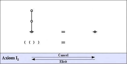
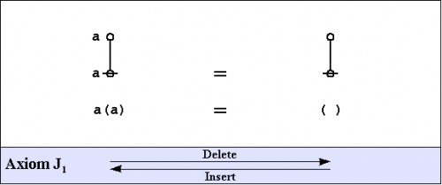
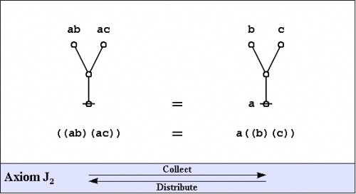
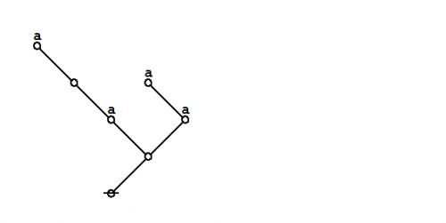
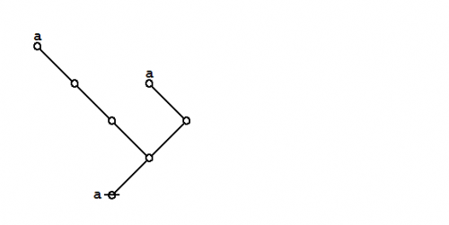
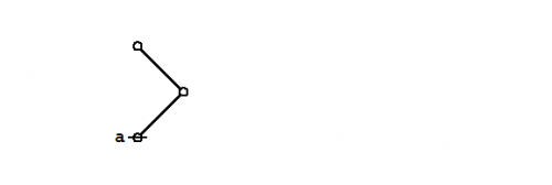
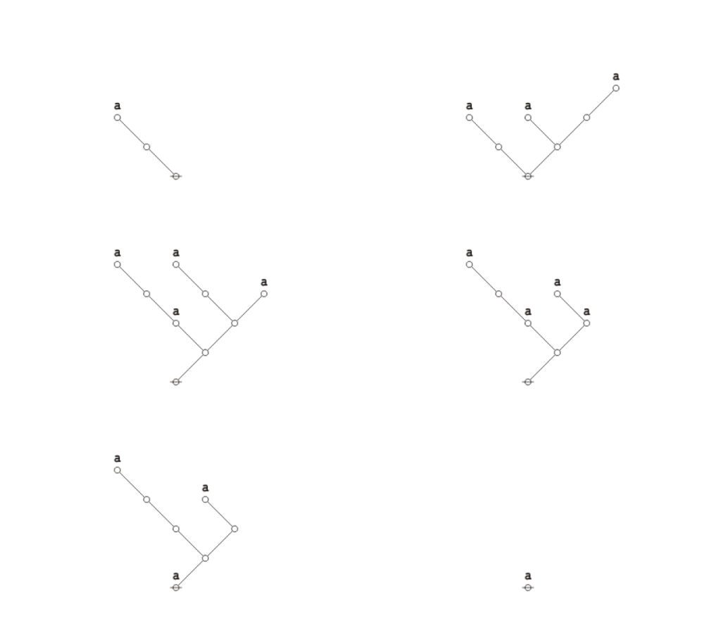
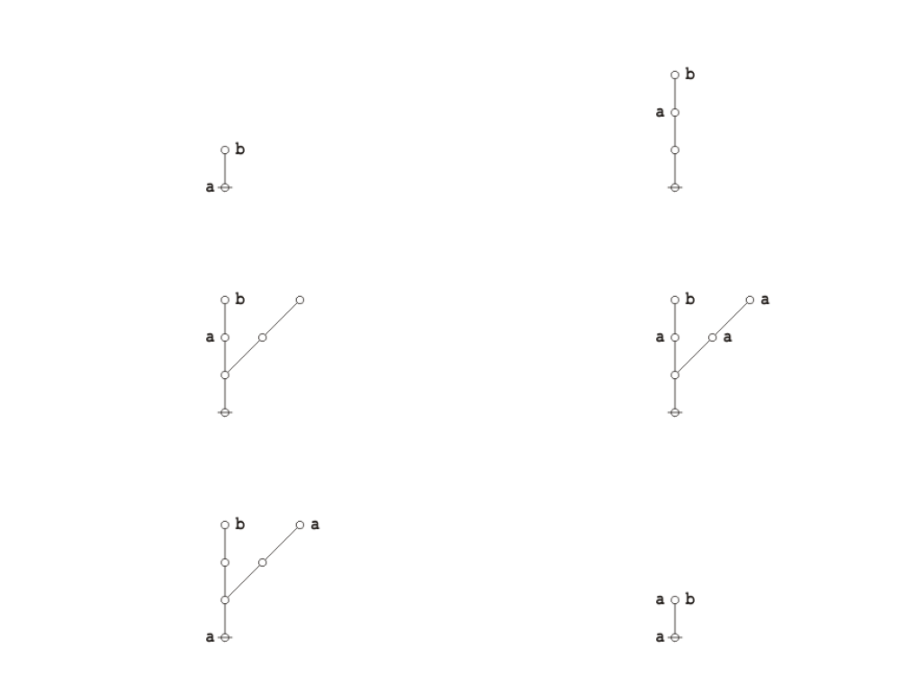
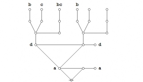
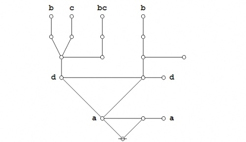
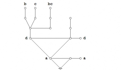
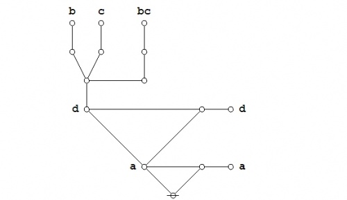
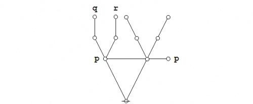
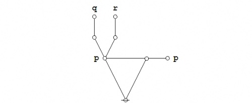
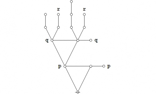
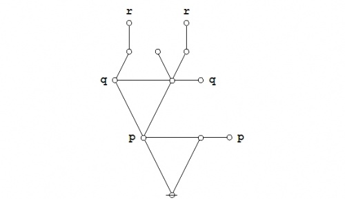
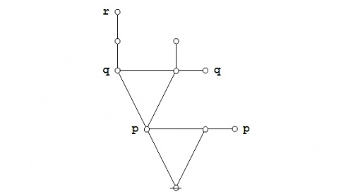
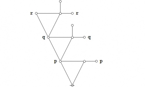
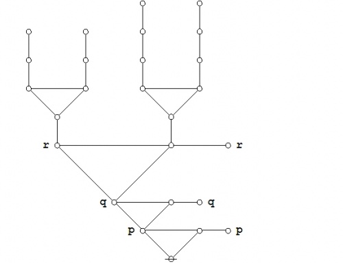
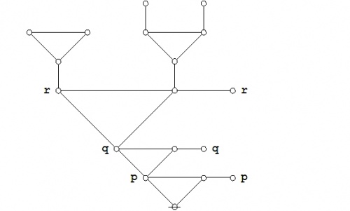
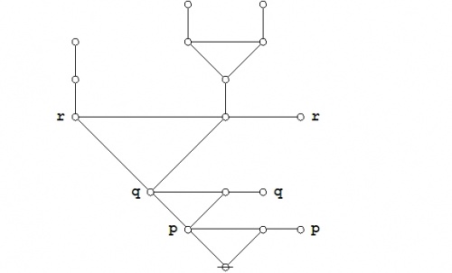
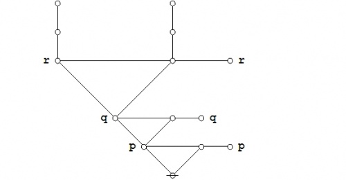
The axioms are just four in number, divided into the arithmetic initials, \(I_1\!\) and \(I_2,\!\) and the algebraic initials, \(J_1\!\) and \(J_2.\!\)
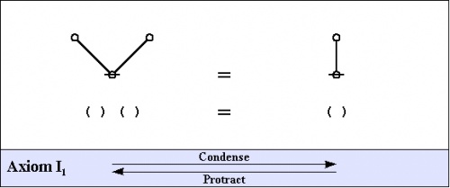
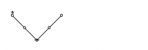
PERS Figure 01.jpg (1)
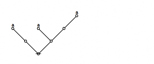
PERS Figure 02.jpg (2)
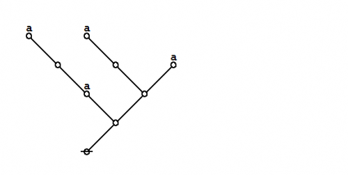
PERS Figure 03.jpg (3)
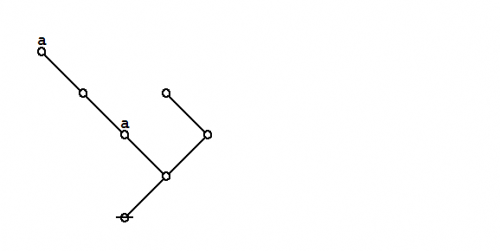
PERS Figure 04.jpg (4)

One way of assigning logical meaning to the initial equations is known as the entitative interpretation (\(\operatorname{En}\)). Under \(\operatorname{En},\) the axioms read as follows:

\(\begin{matrix} I_1 & : & \operatorname{true} ~\operatorname{or}~ \operatorname{true} & = & \operatorname{true} \\ I_2 & : & \operatorname{not}~ \operatorname{true} & = & \operatorname{false} \\ J_1 & : & a ~\operatorname{or}~ \operatorname{not}~ a & = & \operatorname{true} \\ J_2 & : & (a ~\operatorname{or}~ b) ~\operatorname{and}~ (a ~\operatorname{or}~ c) & = & a ~\operatorname{or}~ (b ~\operatorname{and}~ c) \end{matrix}\)

Another way of assigning logical meaning to the initial equations is known as the existential interpretation (\(\operatorname{Ex}\)). Under \(\operatorname{Ex},\) the axioms read as follows:

\(\begin{matrix} I_1 & : & \operatorname{false} ~\operatorname{and}~ \operatorname{false} & = & \operatorname{false} \\ I_2 & : & \operatorname{not}~ \operatorname{false} & = & \operatorname{true} \\ J_1 & : & a ~\operatorname{and}~ \operatorname{not}~ a & = & \operatorname{false} \\ J_2 & : & (a ~\operatorname{and}~ b) ~\operatorname{or}~ (a ~\operatorname{and}~ c) & = & a ~\operatorname{and}~ (b ~\operatorname{or}~ c) \end{matrix}\)

All of the axioms in this set have the form of equations. This means that all of the inference licensed by them are reversible. The proof annotation scheme employed below makes use of a double bar \(\overline{\underline{~~~~~~}}\) to mark this fact, but it will often be left to the reader to decide which of the two possible ways of applying the axiom is the one that is called for in a particular case.

Peirce introduced these formal equations at a level of abstraction that is one step higher than their customary interpretations as propositional calculi, which two readings he called the Entitative and the Existential interpretations, here referred to as \(\operatorname{En}\) and \(\operatorname{Ex},\) respectively. The early CSP, as in his essay on "Qualitative Logic", and also GSB, emphasized the \(\operatorname{En}\) interpretation, while the later CSP developed mostly the \(\operatorname{Ex}\) interpretation.

Frequently used theorems

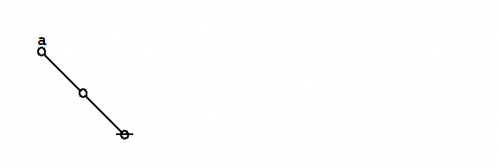
C1. Double negation

The first theorem goes under the names of Consequence 1 \((C_1)\!\), the double negation theorem (DNT), or Reflection.
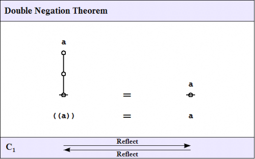
Double Negation 1.0 Splash Page.png (5)

The proof that follows is adapted from the one that was given by George Spencer Brown in his book Laws of Form (LOF) and credited to two of his students, John Dawes and D.A. Utting.

Double Negation 1.0 Marquee Title.png
Double Negation 1.0 Storyboard 1.png
Equational Inference I2 Elicit (( )).png
Double Negation 1.0 Storyboard 2.png
Equational Inference J1 Insert (a).png
Double Negation 1.0 Storyboard 3.png
Equational Inference J2 Distribute ((a)).png
Double Negation 1.0 Storyboard 4.png
Equational Inference J1 Delete (a).png
Double Negation 1.0 Storyboard 5.png
Equational Inference J1 Insert a.png
Double Negation 1.0 Storyboard 6.png
Equational Inference J2 Collect a.png
Double Negation 1.0 Storyboard 7.png
Equational Inference J1 Delete ((a)).png
Double Negation 1.0 Storyboard 8.png
Equational Inference I2 Cancel (( )).png
Double Negation 1.0 Storyboard 9.png
Equational Inference Marquee QED.png
(6)

The steps of this proof are replayed in the following animation.

Double Negation 2.0 Animation.gif
(7)

C2. Generation theorem

One theorem of frequent use goes under the nickname of the weed and seed theorem (WAST). The proof is just an exercise in mathematical induction, once a suitable basis is laid down, and it will be left as an exercise for the reader. What the WAST says is that a label can be freely distributed or freely erased anywhere in a subtree whose root is labeled with that label. The second in our list of frequently used theorems is in fact the base case of this weed and seed theorem. In LOF, it goes by the names of Consequence 2 \((C_2)\!\) or Generation.
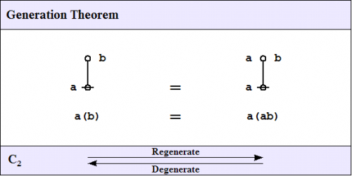
Generation Theorem 1.0 Splash Page.png (8)

Here is a proof of the Generation Theorem.

Generation Theorem 1.0 Marquee Title.png
Generation Theorem 1.0 Storyboard 1.png
Equational Inference C1 Reflect a(b).png
Generation Theorem 1.0 Storyboard 2.png
Equational Inference I2 Elicit (( )).png
Generation Theorem 1.0 Storyboard 3.png
Equational Inference J1 Insert a.png
Generation Theorem 1.0 Storyboard 4.png
Equational Inference J2 Collect a.png
Generation Theorem 1.0 Storyboard 5.png
Equational Inference C1 Reflect a, b.png
Generation Theorem 1.0 Storyboard 6.png
Equational Inference Marquee QED.png
(9)

The steps of this proof are replayed in the following animation.

Generation Theorem 2.0 Animation.gif
(10)

C3. Dominant form theorem

The third of the frequently used theorems of service to this survey is one that Spencer-Brown annotates as Consequence 3 \((C_3)\!\) or Integration. A better mnemonic might be dominance and recession theorem (DART), but perhaps the brevity of dominant form theorem (DFT) is sufficient reminder of its double-edged role in proofs.
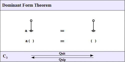
Dominant Form 1.0 Splash Page.png (11)

Here is a proof of the Dominant Form Theorem.

Dominant Form 1.0 Marquee Title.png
Dominant Form 1.0 Storyboard 1.png
Equational Inference C2 Regenerate a.png
Dominant Form 1.0 Storyboard 2.png
Equational Inference J1 Delete a.png
Dominant Form 1.0 Storyboard 3.png
Equational Inference Marquee QED.png
(12)

The following animation provides an instant re*play.

Dominant Form 2.0 Animation.gif
(13)

Exemplary proofs

Based on the axioms given at the outest, and aided by the theorems recorded so far, it is possible to prove a multitude of much more complex theorems. A couple of all-time favorites are given next.

Peirce's law

Main article : Peirce's law

Peirce's law is commonly written in the following form:

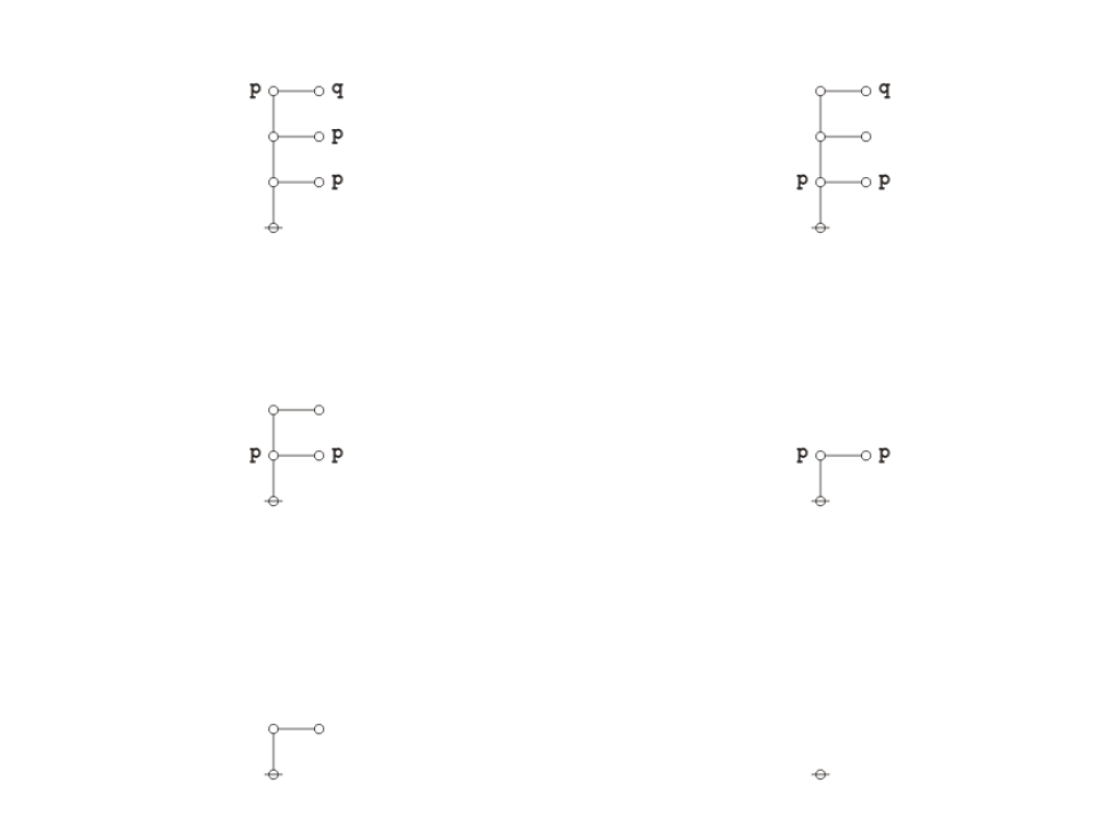
\(((p \Rightarrow q) \Rightarrow p) \Rightarrow p\)

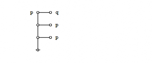
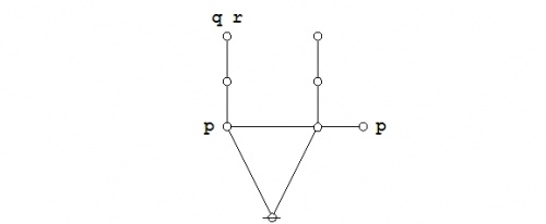
The existential graph representation of Peirce's law is shown below.
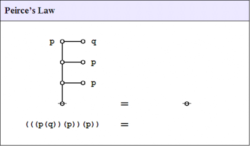
Peirce's Law 1.0 Splash Page.png (14)

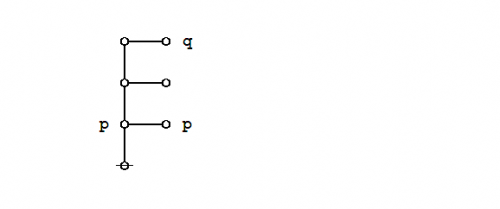
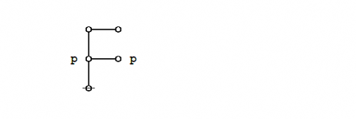
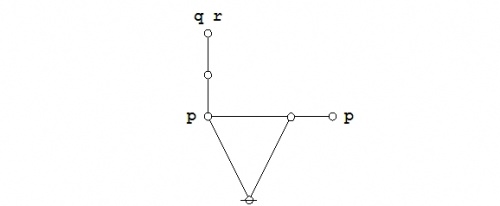
A graphical proof of Peirce's law is shown next.

Peirce's Law 1.0 Marquee Title.png
Peirce's Law 1.0 Storyboard 1.png
Equational Inference Band Collect p.png
Peirce's Law 1.0 Storyboard 2.png
Equational Inference Band Quit ((q)).png
Peirce's Law 1.0 Storyboard 3.png
Equational Inference Band Cancel (( )).png
Peirce's Law 1.0 Storyboard 4.png
Equational Inference Band Delete p.png
Peirce's Law 1.0 Storyboard 5.png
Equational Inference Band Cancel (( )).png
Peirce's Law 1.0 Storyboard 6.png
Equational Inference Marquee QED.png
(15)

The following animation replays the steps of the proof.

Peirce's Law 2.0 Animation.gif
(16)

Praeclarum theorema

An illustrious example of a propositional theorem is the praeclarum theorema, the admirable, shining, or splendid theorem of Leibniz.

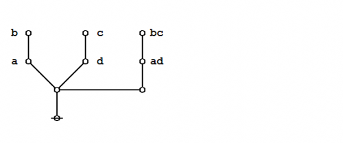
If a is b and d is c, then ad will be bc.

This is a fine theorem, which is proved in this way:

a is b, therefore ad is bd (by what precedes),

d is c, therefore bd is bc (again by what precedes),

ad is bd, and bd is bc, therefore ad is bc. Q.E.D.

(Leibniz, Logical Papers, p. 41).

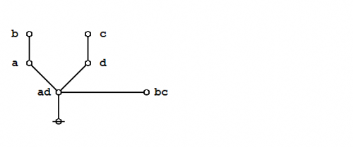
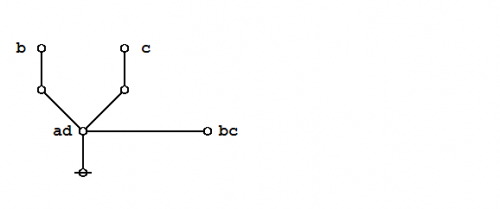
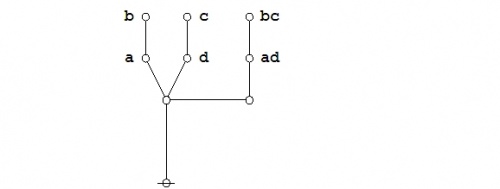
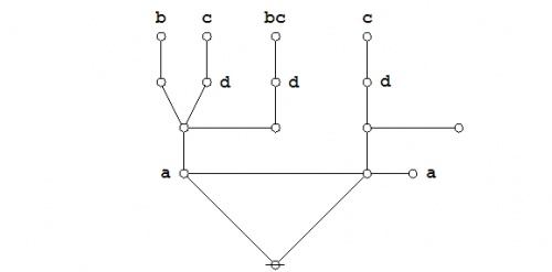
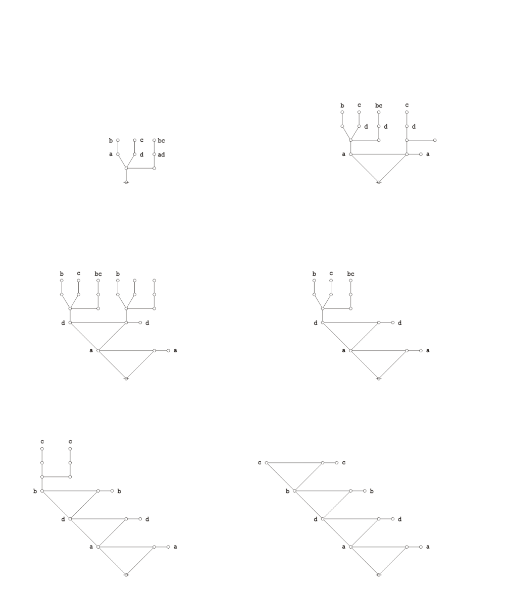
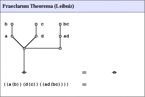
Under the existential interpretation, the praeclarum theorema is represented by means of the following logical graph.
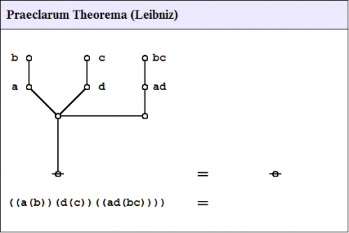
Praeclarum Theorema 1.0 Splash Page.png (17)

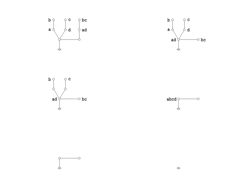
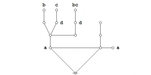
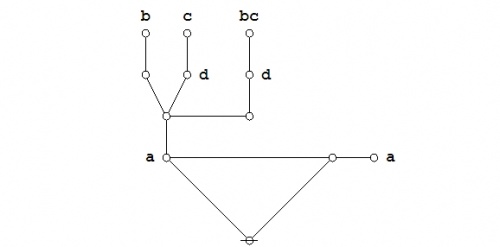
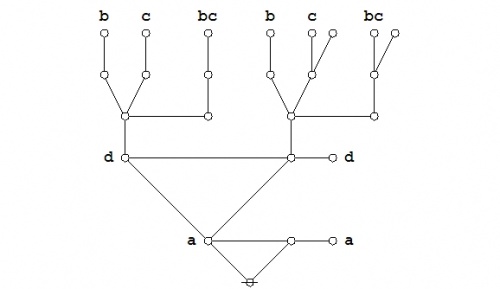
And here's a neat proof of that nice theorem.

Praeclarum Theorema 1.0 Marquee Title.png
Praeclarum Theorema 1.0 Storyboard 1.png
Equational Inference Rule Reflect ad(bc).png
Praeclarum Theorema 1.0 Storyboard 2.png
Equational Inference Rule Weed a, d.png
Praeclarum Theorema 1.0 Storyboard 3.png
Equational Inference Rule Reflect b, c.png
Praeclarum Theorema 1.0 Storyboard 4.png
Equational Inference Rule Weed bc.png
Praeclarum Theorema 1.0 Storyboard 5.png
Equational Inference Rule Quit abcd.png
Praeclarum Theorema 1.0 Storyboard 6.png
Equational Inference Rule Cancel (( )).png
Praeclarum Theorema 1.0 Storyboard 7.png
Equational Inference Marquee QED.png
(18)

The steps of the proof are replayed in the following animation.

Praeclarum Theorema 2.0 Animation.gif
(19)

Two-thirds majority function

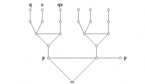
Consider the following equation in boolean algebra, posted as a problem for proof at MathOverFlow.

\(\begin{matrix} a b \bar{c} + a \bar{b} c + \bar{a} b c + a b c \'"`UNIQ-MathJax1-QINU`"'  \(\texttt{(\_, \_)},\)  \(\texttt{(\_, \_, \_)},\)  and so on, where the number of argument slots is the order of the reflective negation operator in question.

The formal rule of evaluation for a \(k\!\)-lobe or \(k\!\)-operator may be summarized as follows:

o-----------------------------------------------------------o
| Evaluation Rule                                           |
o-----------------------------------------------------------o
|                                                           |
|     x_1  x_2   ...  x_k                                   |
|      o----o-...-o----o                                    |
|       \             /                                     |
|        \           /                                      |
|         \         /                                       |
|          \       /                                        |
|           \     /                                         |
|            \   /                                          |
|             \ /                                           |
|              @              =              @              |
|                                                           |
|                                                           |
|   ( x_1, x_2, ..., x_k )    =           <space>           |
|                                                           |
|                                                           |
|                       IF AND ONLY IF                      |
|                                                           |
|                                            o              |
|   Just one of the x_1, x_2, ..., x_k   =   |   =   ( )    |
|                                            @              |
|                                                           |
o-----------------------------------------------------------o
(1)

The interpretation of these operators, read as assertions about the values of their listed arguments, is as follows:

o-----------------------------------------------------------o
| Interpretation Rule                                       |
o-----------------------------------------------------------o
|                                                           |
|               x_1  x_2   ...  x_k                         |
|                o----o-...-o----o                          |
|                 \             /                           |
|                  \           /                            |
|                   \         /                             |
|                    \       /                              |
|                     \     /                               |
|                      \   /                                |
|                       \ /                                 |
|                        @                                  |
|                                                           |
|                                                           |
| A "k-lobe operator" of the form "(x_1, ..., x_k)"         |
| enjoys two commonly employed interpretations for          |
| propositional logic, in other words, two ways of          |
| taking it as an assertion about, or a constraint          |
| upon, the logical values of the listed arguments,         |
| the mentioned variables x_j, for j = 1 through k.         |
|                                                           |
| Existential Interpretation:                               |
|                                                           |
|    "Just one of the k arguments is not true."             |
|                                                           |
| Entitative  Interpretation:                               |
|                                                           |
|    "Not just one of the k arguments is true."             |
|                                                           |
o-----------------------------------------------------------o
(2)

Case analysis-synthesis theorem

Discusssion

The task at hand is build a bridge between model-theoretic and proof-theoretic perspectives on logical procedure, though for now we join them at a point so close to their common source that it may not seem worth the candle at all. The substance of this principle was known to Boole in the 1850's, tantamount to what we now call the boolean expansion of a propositional expression. The only novelty here resides in a certain manner of presentation, in which we will prove the basic principle from the axioms given before. One name for this rule is the Case Analysis-Synthesis Theorem (CAST).

I am going to revert to my customarily sloppy workshop manners and refer to propositions and proposition expressions on rough analogy with functions and function expressions, which implies that a proposition will be regarded as the chief formal object of discussion, enjoying many proposition expressions, formulas, or sentences that express it, but worst of all I will probably just go ahead and use any and all of these terms as loosely as I see fit, taking a bit of extra care only when I see the need.

Let \(Q\!\) be a propositional expression with an unspecified, but context-appropriate number of variables, say, none, or \(x,\!\) or \(x_1, \ldots, x_k,\!\) as the case may be.

  • Strings and graphs that have no labels are called bare.
  • A bare terminal node, symbolized by a small circle \(\circ\) in text, is known as a stone.
  • A bare terminal edge, symbolized by a vertical bar \(\vert\) in text, is known as a stick.

Let the replacement expression of the form \(Q[\circ /x]\) denote the proposition that results from \(Q\!\) by replacing every token of the variable \(x\!\) with a blank, that is to say, by erasing \(x.\!\)

Let the replacement expression of the form \(Q[\,\vert /x]\) denote the proposition that results from \(Q\!\) by replacing every token of the variable \(x\!\) with a stick stemming from the site of \(x.\!\)

In the case of a propositional expression \(Q\!\) that has no token of the designated variable \(x,\!\) let it be stipulated that \(Q[\circ /x] = Q = Q[\,\vert /x].\)

I think that I am at long last ready to state the following:

o-----------------------------------------------------------o
| Case Analysis-Synthesis Theorem (CAST)                    |
o-----------------------------------------------------------o
|                                                           |
|                                              x            |
|                                              o            |
|                                          x   |            |
|                                   Q[o/x] o---o Q[|/x]     |
|              Q                            \ /             |
|              @              =              @              |
|                                                           |
o-----------------------------------------------------------o
|                                                           |
|              Q              =   ( Q[o/x] x , Q[|/x] (x) ) |
|                                                           |
o-----------------------------------------------------------o
(1)

In order to think of tackling even the roughest sketch toward a proof of this theorem, we need to add a number of axioms and axiom schemata. Because I abandoned proof-theoretic purity somewhere in the middle of grinding this calculus into computational form, I never got around to finding the most elegant and minimal, or anything near a complete set of axioms for the cactus language, so what I list here are just the slimmest rudiments of the hodge-podge of rules of thumb that I have found over time to be necessary and useful in most working settings. Some of these special precepts are probably provable from genuine axioms, but I have yet to go looking for a more proper formulation.

o-----------------------------------------------------------o
| Precept L_1.  Indifference                                |
o-----------------------------------------------------------o
|                                                           |
|                     a                                     |
|                     o                                     |
|                 a   |                                     |
|                 o---o                                     |
|                  \ /                                      |
|                   @         =         @                   |
|                                                           |
o-----------------------------------------------------------o
|                                                           |
|                (a, (a))     =                             |
|                                                           |
o-----------------------------------------------------------o
|                 Split <---- | ----> Merge                 |
o-----------------------------------------------------------o
(2)
 
o-----------------------------------------------------------o
| Precept L_2.  Equality.  The Following Are Equivalent:    |
o-----------------------------------------------------------o
|                                                           |
|           b               a   b               a           |
|           o               o---o               o           |
|       a   |                \ /                |   b       |
|       o---o                 o                 o---o       |
|        \ /                  |                  \ /        |
|         @         =         @         =         @         |
|                                                           |
o-----------------------------------------------------------o
|                                                           |
|      (a, (b))     =     ((a , b))     =     ((a), b)      |
|                                                           |
o-----------------------------------------------------------o
(3)
 
o-----------------------------------------------------------o
| Precept L_3.  Dispersion                                  |
o-----------------------------------------------------------o
|                                                           |
| For k > 1, the following equation holds:                  |
|                                                           |
|   y_1    y_2   ...    y_k     x y_1  x y_2   ...  x y_k   |
|    o------o-...-o------o         o------o-...-o------o    |
|     \                 /           \                 /     |
|      \               /             \               /      |
|       \             /               \             /       |
|        \           /                 \           /        |
|         \         /                   \         /         |
|          \       /                     \       /          |
|           \     /                       \     /           |
|            \   /                         \   /            |
|             \ /                           \ /             |
|            x @              =              @              |
|                                                           |
|     x (y_1, ..., y_k)       =     (x y_1, ..., x y_k)     |
|                                                           |
o-----------------------------------------------------------o
|           Distill     <---- | ---->     Disperse          |
o-----------------------------------------------------------o
(4)

To see why the Dispersion Rule holds, look at it this way: If \(x\!\) is true, then the presence of \(x\!\) makes no difference on either side of the equation, but if \(x\!\) is false, then both sides of the equation are false.

Here is a proof sketch for the Case Analysis-Synthesis Theorem (CAST):

o-----------------------------------------------------------o
| Case Analysis-Synthesis Theorem.  Proof Sketch.           |
o-----------------------------------------------------------o
|                                                           |
|              Q                                            |
|              @                                            |
|                                                           |
o=============================< L1. Split " " >=============o
|                                                           |
|                x                                          |
|                o                                          |
|            x   |                                          |
|            o---o                                          |
|             \ /                                           |
|            Q @                                            |
|                                                           |
o=============================< L3. Disperse "Q" >==========o
|                                                           |
|                x                                          |
|                o                                          |
|            x   |                                          |
|          Q o---o Q                                        |
|             \ /                                           |
|              @                                            |
|                                                           |
o=============================< C1. Reflect "x" >===========o
|                                                           |
|                x                                          |
|                o                                          |
|            x   |                                          |
|          Q o---o Q[((x))/x]                               |
|             \ /                                           |
|              @                                            |
|                                                           |
o=============================< C2. Weed "x", "(x)" >=======o
|                                                           |
|                x                                          |
|                o                                          |
|            x   |                                          |
|     Q[o/x] o---o Q[|/x]                                   |
|             \ /                                           |
|              @                                            |
|                                                           |
o=============================< QES >=======================o
(5)

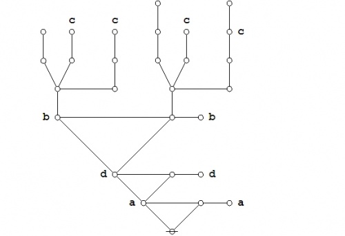
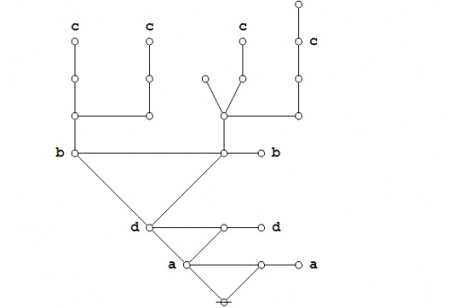
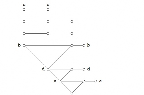
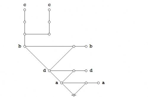
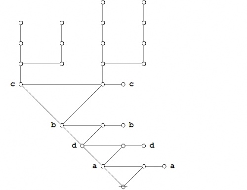
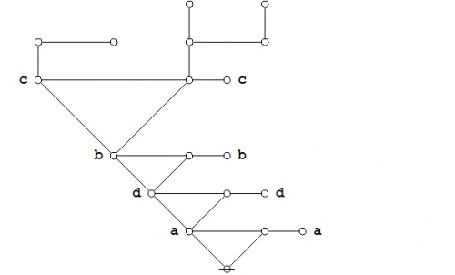
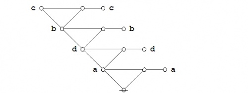
Praeclarum theorema : Proof by CAST

Some of the jobs that the CAST can be put to work on are proving propositional theorems and establishing equations between propositions. Once again, let us turn to the example of Leibniz's Praeclarum Theorema as a way of illustrating how.

Proof Praeclarum Theorema CAST 00.jpg
Proof Praeclarum Theorema CAST 01.jpg
Equational Inference Bar -- Cast A.jpg
Proof Praeclarum Theorema CAST 02.jpg
Equational Inference Bar -- Domination.jpg
Proof Praeclarum Theorema CAST 03.jpg
Equational Inference Bar -- Cancellation.jpg
Proof Praeclarum Theorema CAST 04.jpg
Equational Inference Bar -- Domination.jpg
Proof Praeclarum Theorema CAST 05.jpg
Equational Inference Bar -- Cancellation.jpg
Proof Praeclarum Theorema CAST 06.jpg
Equational Inference Bar -- Cast D.jpg
Proof Praeclarum Theorema CAST 07.jpg
Equational Inference Bar -- Domination.jpg
Proof Praeclarum Theorema CAST 08.jpg
Equational Inference Bar -- Cancellation.jpg
Proof Praeclarum Theorema CAST 09.jpg
Equational Inference Bar -- Domination.jpg
Proof Praeclarum Theorema CAST 10.jpg
Equational Inference Bar -- Cancellation.jpg
Proof Praeclarum Theorema CAST 11.jpg
Equational Inference Bar -- Cast B.jpg
Proof Praeclarum Theorema CAST 12.jpg
Equational Inference Bar -- Cancellation.jpg
Proof Praeclarum Theorema CAST 13.jpg
Equational Inference Bar -- Domination.jpg
Proof Praeclarum Theorema CAST 14.jpg
Equational Inference Bar -- Cancellation.jpg
Proof Praeclarum Theorema CAST 15.jpg
Equational Inference Bar -- Cast C.jpg
Proof Praeclarum Theorema CAST 16.jpg
Equational Inference Bar -- Cancellation.jpg
Proof Praeclarum Theorema CAST 17.jpg
Equational Inference Bar -- Cancellation.jpg
Proof Praeclarum Theorema CAST 18.jpg
Equational Inference Bar -- QED.jpg
(1)

The following Figure provides an animated recap of the graphical transformations that occur in the above proof:

Praeclarum Theorema CAST 500 x 389 Animation.gif
(2)

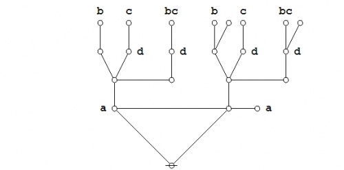
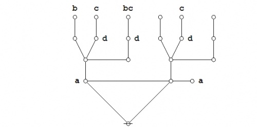
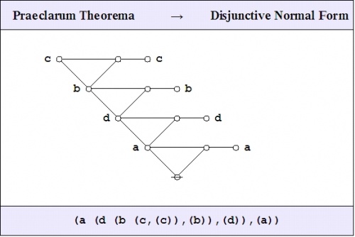
The logical graph that concludes this proof is a variant type of disjunctive normal form (DNF) for the logical graph that was to be demonstrated.

Praeclarum Theorema DNF.jpg (3)

Remembering that a blank node is the graphical equivalent of a logical value \(\operatorname{true},\) the resulting DNF may be read as follows:

o-----------------------------------------------------------o
|                                                           |
| Either not 'a' and thus 'true'                            |
|     Or     'a' and thus                                   |
|        Either not 'd' and thus 'true'                     |
|            Or     'd' and thus                            |
|               Either not 'b' and thus 'true'              |
|                   Or     'b' and thus                     |
|                      Either not 'c' and thus 'true'       |
|                          Or     'c' and thus true.        |
|                                                           |
o-----------------------------------------------------------o
(4)

That is tantamount to saying that the proposition being submitted for analysis is true in every case. Thus we are justified in awarding it the title of a Theorem.

Logic as sign transformation

We have been looking at various ways of transforming propositional expressions, expressed in the parallel formats of character strings and graphical structures, all the while preserving certain aspects of their "meaning" — and here I risk using that vaguest of all possible words, but only as a promissory note, hopefully to be cached out in a more meaningful species of currency as the discussion develops.

I cannot pretend to be acquainted with or to comprehend every form of intension that others might find of interest in a given form of expression, nor can I speak for every form of meaning that another might find in a given form of syntax. The best that I can hope to do is to specify what my object is in using these expressions, and to say what aspects of their syntax are meant to serve this object, lending these properties the interest I have in preserving them as I put the expressions through the paces of their transformations.

On behalf of this object I have been spinning in the form of this thread a developing example base of propositional expressions, in the data structures of graphs and strings, along with many examples of step-wise transformations on these expressions that preserve something of significant logical import, something that might be referred to as their logical equivalence class (LEC), and that we could as well call the constraint information or the denotative object of the expression in view.

To focus still more, let us return to that Splendid Theorem noted by Leibniz, and let us look more carefully at the two distinct ways of transforming its initial expression that we just used to arrive at an equivalent expression, one that made its tautologous character or its theorematic nature as evident as it could be.

Just to remind you, here is the Splendid Theorem again:

Praeclarum Theorema.jpg (1)
The first way of transforming the expression that appears on the left hand side of the equation can be described as proof-theoretic in character.
The second way of transforming the expression that appears on the left hand side of the equation can be described as model-theoretic in character.

What we have here amounts to a couple of different styles of communicative conduct, that is, two sequences of signs of the form \(e_1, e_2, \ldots, e_n,\!\) each one beginning with a problematic expression and eventually ending with a clear expression of the logical equivalence class to which every sign or expression in the sequence belongs. Ordinarily, any orbit through a locus of signs can be taken to reflect an underlying sign-process, a case of semiosis. So what we have here are two very special cases of semiosis, and what we may find it useful to contemplate is how to characterize them as two species of a very general class.

We are starting to delve into some fairly picayune details of a particular sign system, non-trivial enough in its own right but still rather simple compared to the types of our ultimate interest, and though I believe that this exercise will be worth the effort in prospect of understanding more complicated sign systems, I feel that I ought to say a few words about the larger reasons for going through this work.

My broader interest lies in the theory of inquiry as a special application or a special case of the theory of signs. Another name for the theory of inquiry is logic and another name for the theory of signs is semiotics. So I might as well have said that I am interested in logic as a special application or a special case of semiotics. But what sort of a special application? What sort of a special case? Well, I think of logic as formal semiotics — though, of course, I am not the first to have said such a thing — and by formal we say, in our etymological way, that logic is concerned with the form, indeed, with the animate beauty and the very life force of signs and sign actions. Yes, perhaps that is far too Latin a way of understanding logic, but it's all I've got.

Now, if you think about these things just a little more, I know that you will find them just a little suspicious, for what besides logic would I use to do this theory of signs that I would apply to this theory of inquiry that I'm also calling logic? But that is precisely one of the things signified by the word formal, for what I'd be required to use would have to be some brand of logic, that is, some sort of innate or inured skill at inquiry, but a style of logic that is casual, catch-as-catch-can, formative, incipient, inchoate, unformalized, a work in progress, partially built into our natural language and partially more primitive than our most artless language. In so far as I use it more than mention it, mention it more than describe it, and describe it more than fully formalize it, then to that extent it must be consigned to the realm of unformalized and unreflective logic, where some say "there be oracles", but I don't know.

Still, one of the aims of formalizing what acts of reasoning that we can is to draw them into an arena where we can examine them more carefully, perhaps to get better at their performance than we can unreflectively, and thus to live, to formalize again another day. Formalization is not the be-all end-all of human life, not by a long shot, but it has its uses on that behalf.

This looks like a good place to pause and take stock. The question arises: What is really going on here? We have all these signs, but what is the object? One object worth the candle is simply to study a non-trivial example of a syntactic system, simple in design but not entirely a toy, just to see how these systems tick. More than that, we would like to understand how sign systems come to exist or can be placed in relation to object systems, in the likes of which we possess some compelling independent reason to take an interest. What is the utility of setting up sets of strings and sets of graphs, and sorting them according to their semiotic equivalence class (SEC) based on this or that abstract notion of transformational equivalence?

Good questions.

I can but begin to address these questions in the present frame of work, but I can't hope to answer them in anything like a satisfactory fashion. Nevertheless, I will not mind one bit if you keep them in mind as we go.

Analysis of contingent propositions

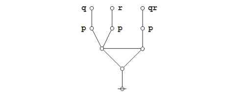
For all of the reasons mentioned above, and for the sake of a more compact illustration of the ins and outs of a typical propositional equation reasoning system, let's now take up a much simpler example of a contingent proposition:

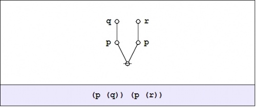
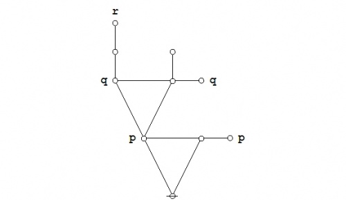
Logical Graph (P (Q)) (P (R)).jpg (1)

For the sake of simplicity in discussing this example, let's stick with the existential interpretation (\(\operatorname{Ex}\)) of logical graphs and their corresponding parse strings. Under \(\operatorname{Ex}\) the formal expression \(\texttt{(} p \texttt{(} q \texttt{))(} p \texttt{(} r \texttt{))}\) translates into the vernacular expression \({}^{\backprime\backprime} p ~\operatorname{implies}~ q ~\operatorname{and}~ p ~\operatorname{implies}~ r {}^{\prime\prime},\) in symbols, \((p \Rightarrow q) \land (p \Rightarrow r),\) so this is the reading that we'll want to keep in mind for the present. Where brevity is required, we may refer to the propositional expression \(\texttt{(} p \texttt{(} q \texttt{))(} p \texttt{(} r \texttt{))}\) under the name \(f\!\) by making use of the following definition:

\(f ~=~ \texttt{(} p \texttt{(} q \texttt{))(} p \texttt{(} r \texttt{))}\)

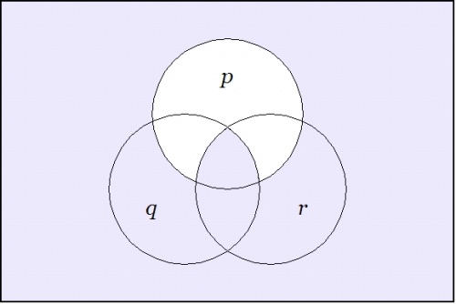
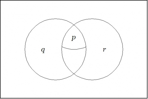
Since the expression \(\texttt{(} p \texttt{(} q \texttt{))(} p \texttt{(} r \texttt{))}\) involves just three variables, it may be worth the trouble to draw a venn diagram of the situation. There are in fact two different ways to execute the picture.

Figure 2 indicates the points of the universe of discourse \(X\!\) for which the proposition \(f : X \to \mathbb{B}\) has the value 1, here interpreted as the logical value \(\operatorname{true}.\) In this paint by numbers style of picture, one simply paints over the cells of a generic template for the universe \(X,\!\) going according to some previously adopted convention, for instance: Let the cells that get the value 0 under \(f\!\) remain untinted and let the cells that get the value 1 under \(f\!\) be painted or shaded. In doing this, it may be good to remind ourselves that the value of the picture as a whole is not in the paints, in other words, the \(0, 1\!\) in \(\mathbb{B},\) but in the pattern of regions that they indicate.

Venn Diagram (P (Q)) (P (R)).jpg (2)
\(\text{Venn Diagram for}~ \texttt{(} p \texttt{~(} q \texttt{))~(} p \texttt{~(} r \texttt{))}\)

There are a number of standard ways in mathematics and statistics for talking about the subset \(W\!\) of the functional domain \(X\!\) that gets painted with the value \(z \in \mathbb{B}\) by the indicator function \(f : X \to \mathbb{B}.\) The region \(W \subseteq X\) is called by a variety of names in different settings, for example, the antecedent, the fiber, the inverse image, the level set, or the pre-image in \(X\!\) of \(z\!\) under \(f.\!\) It is notated and defined as \(W = f^{-1}(z).\!\) Here, \(f^{-1}\!\) is called the converse relation or the inverse relation — it is not in general an inverse function — corresponding to the function \(f.\!\) Whenever possible in simple examples, we use lower case letters for functions \(f : X \to \mathbb{B},\) and it is sometimes useful to employ capital letters for subsets of \(X,\!\) if possible, in such a way that \(F\!\) is the fiber of 1 under \(f,\!\) in other words, \(F = f^{-1}(1).\!\)

The easiest way to see the sense of the venn diagram is to notice that the expression \(\texttt{(} p \texttt{(} q \texttt{))},\) read as \(p \Rightarrow q,\) can also be read as \({}^{\backprime\backprime} \operatorname{not}~ p ~\operatorname{without}~ q {}^{\prime\prime}.\) Its assertion effectively excludes any tincture of truth from the region of \(P\!\) that lies outside the region \(Q.\!\) In a similar manner, the expression \(\texttt{(} p \texttt{(} r \texttt{))},\) read as \(p \Rightarrow r,\) can also be read as \({}^{\backprime\backprime} \operatorname{not}~ p ~\operatorname{without}~ r {}^{\prime\prime}.\) Asserting it effectively excludes any tincture of truth from the region of \(P\!\) that lies outside the region \(R.\!\)

Figure 3 shows the other standard way of drawing a venn diagram for such a proposition. In this punctured soap film style of picture — others may elect to give it the more dignified title of a logical quotient topology — one begins with Figure 31 and then proceeds to collapse the fiber of 0 under \(X\!\) down to the point of vanishing utterly from the realm of active contemplation, arriving at the following picture:

Venn Diagram (P (Q R)).jpg (3)
\(\text{Venn Diagram for}~ \texttt{(} p \texttt{~(} q ~ r \texttt{))}\)

This diagram indicates that the region where \(p\!\) is true is wholly contained in the region where both \(q\!\) and \(r\!\) are true. Since only the regions that are painted true in the previous figure show up at all in this one, it is no longer necessary to distinguish the fiber of 1 under \(f\!\) by means of any shading.

In sum, it is immediately obvious from the venn diagram that in drawing a representation of the following propositional expression:

\(\texttt{(} p \texttt{(} q \texttt{))(} p \texttt{(} r \texttt{))},\)

in other words,

\((p \Rightarrow q) \land (p \Rightarrow r),\)

we are also looking at a picture of:

\(\texttt{(} p \texttt{(} q r \texttt{))},\)

in other words,

\(p \Rightarrow (q \land r).\)

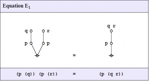
Let us now examine the following propositional equation:

Logical Graph (P (Q)) (P (R)) = (P (Q R)).jpg (4)

There are three distinct ways that I can think of right off as to how we might go about formally proving or systematically checking the proposed equivalence, the evidence of whose truth we already have before us clearly enough, and in a visually intuitive form, from the venn diagrams that we examined above.

While we go through each of these ways let us keep one eye out for the character and the conduct of each type of proceeding as a semiotic process, that is, as an orbit, in this case discrete, through a locus of signs, in this case propositional expressions, and as it happens in this case, a sequence of transformations that perseveres in the denotative objective of each expression, that is, in the abstract proposition that it expresses, while it preserves the informed constraint on the universe of discourse that gives us one viable candidate for the informational content of each expression in the interpretive chain of sign metamorphoses.

A sign relation \(L\!\) is a subset of a cartesian product \(O \times S \times I,\) where \(O, S, I\!\) are sets known as the object, sign, and interpretant sign domains, respectively. These facts are symbolized by writing \(L \subseteq O \times S \times I.\) Accordingly, a sign relation \(L\!\) consists of ordered triples of the form \((o, s, i),\!\) where \(o, s, i\!\) belong to the domains \(O, S, I,\!\) respectively. An ordered triple of the form \((o, s, i) \in L\) is referred to as a sign triple or an elementary sign relation.

The syntactic domain of a sign relation \(L \subseteq O \times S \times I\) is defined as the set-theoretic union \(S \cup I\) of its sign domain \(S\!\) and its interpretant domain \(I.\!\) It is not uncommon, especially in formal examples, for the sign domain and the interpretant domain to be equal as sets, in short, to have \(S = I.\!\)

Sign relations may contain any number of sign triples, finite or infinite. Finite sign relations do arise in applications and can be very instructive as expository examples, but most of the sign relations of significance in logic have infinite sign and interpretant domains, and usually infinite object domains, in the long run, at least, though one frequently works up to infinite domains by a series of finite approximations and gradual stages.

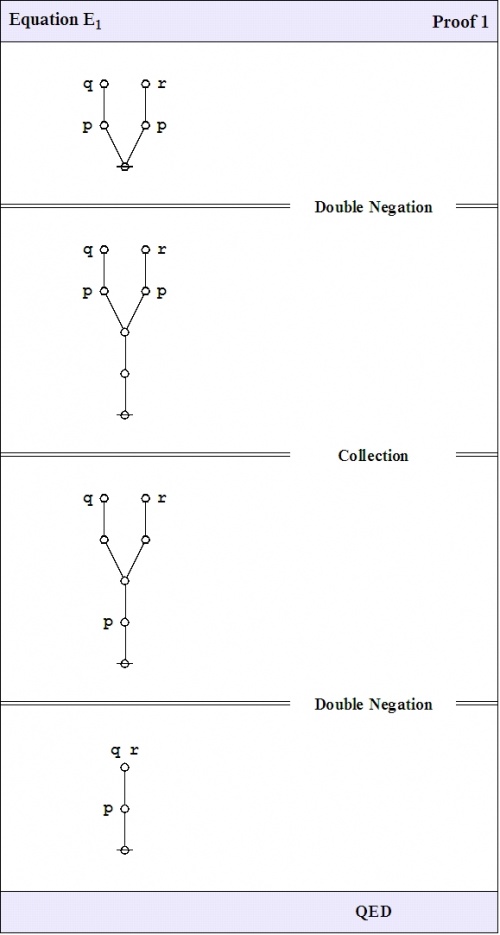
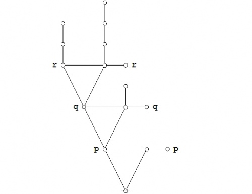
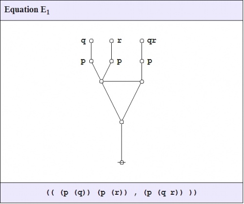
With that preamble behind us, let us turn to consider the case of semiosis, or sign transformation process, that is generated by our first proof of the propositional equation \(E_1.\!\)

Logical Graph (P (Q)) (P (R)) = (P (Q R)) Proof 1.jpg (5)

For some reason I always think of this as the way that our DNA would prove it.

We are in the process of examining various proofs of the propositional equation \(\texttt{(} p \texttt{(} q \texttt{))(} p \texttt{(} r \texttt{))} = \texttt{(} p \texttt{(} q r \texttt{))},\) and viewing these proofs in the light of their character as semiotic processes, in essence, as sign-theoretic transformations.

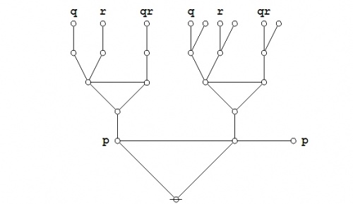
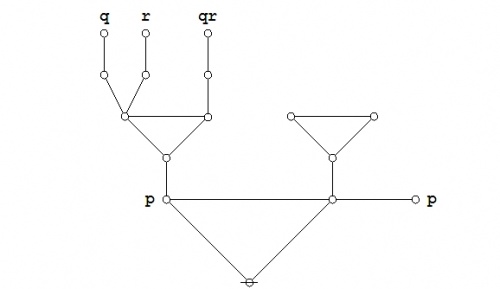
The second way of establishing the truth of this equation is one that I see, rather loosely, as model-theoretic, for no better reason than the sense of its ending with a pattern of expression, a variant of the disjunctive normal form (DNF), that is commonly recognized to be the form that one extracts from a truth table by pulling out the rows of the table that evaluate to true and constructing the disjunctive expression that sums up the senses of the corresponding interpretations.

In order to apply this model-theoretic method to an equation between a couple of contingent expressions, one must transform each expression into its associated DNF and then compare those to see if they are equal. In the current setting, these DNF's may indeed end up as identical expressions, but it is possible, also, for them to turn out slightly off-kilter from each other, and so the ultimate comparison may not be absolutely immediate. The explanation of this is that, for the sake of computational efficiency, it is useful to tailor the DNF that gets developed as the output of a DNF algorithm to the particular form of the propositional expression that is given as input.

Proof (P (Q)) (P (R)) = (P (Q R)) 2-1-0.jpg
Proof (P (Q)) (P (R)) = (P (Q R)) 2-1-1.jpg
Equational Inference Bar -- Cast P.jpg
Proof (P (Q)) (P (R)) = (P (Q R)) 2-1-2.jpg
Equational Inference Bar -- Domination.jpg
Proof (P (Q)) (P (R)) = (P (Q R)) 2-1-3.jpg
Equational Inference Bar -- Cancellation.jpg
Proof (P (Q)) (P (R)) = (P (Q R)) 2-1-4.jpg
Equational Inference Bar -- Cast Q.jpg
Proof (P (Q)) (P (R)) = (P (Q R)) 2-1-5.jpg
Equational Inference Bar -- Cancellation.jpg
Proof (P (Q)) (P (R)) = (P (Q R)) 2-1-6.jpg
Equational Inference Bar -- Domination.jpg
Proof (P (Q)) (P (R)) = (P (Q R)) 2-1-7.jpg
Equational Inference Bar -- Cast R.jpg
Proof (P (Q)) (P (R)) = (P (Q R)) 2-1-8.jpg
Equational Inference Bar -- Cancellation.jpg
Proof (P (Q)) (P (R)) = (P (Q R)) 2-1-9.jpg
Equational Inference Bar -- DNF.jpg
(6)

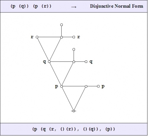
The final graph in the sequence of equivalents is a disjunctive normal form (DNF) for the proposition on the left hand side of the equation \(\texttt{(} p \texttt{(} q \texttt{))(} p \texttt{(} r \texttt{))} = \texttt{(} p \texttt{(} q r \texttt{))}.\)

Logical Graph (P (Q)) (P (R)) DNF.jpg (7)

Remembering that a blank node is the graphical equivalent of a logical value \(\operatorname{true},\) the resulting DNF may be read as follows:

o-----------------------------------------------------------o
|                                                           |
| Either not 'p' and thus 'true'                            |
|     Or     'p' and thus                                   |
|        Either not 'q' and thus 'false'                    |
|            Or     'q' and thus                            |
|               Either not 'r' and thus 'false'             |
|                   Or     'r' and thus 'true'.             |
|                                                           |
o-----------------------------------------------------------o
(8)

It remains to show that the right hand side of the equation \(\texttt{(} p \texttt{(} q \texttt{))(} p \texttt{(} r \texttt{))} = \texttt{(} p \texttt{(} q r \texttt{))}\) is logically equivalent to the DNF just obtained. The needed chain of equations is as follows:

Proof (P (Q)) (P (R)) = (P (Q R)) 2-2-0.jpg
Proof (P (Q)) (P (R)) = (P (Q R)) 2-2-1.jpg
Equational Inference Bar -- Cast P.jpg
Proof (P (Q)) (P (R)) = (P (Q R)) 2-2-2.jpg
Equational Inference Bar -- Domination.jpg
Proof (P (Q)) (P (R)) = (P (Q R)) 2-2-3.jpg
Equational Inference Bar -- Cancellation.jpg
Proof (P (Q)) (P (R)) = (P (Q R)) 2-2-4.jpg
Equational Inference Bar -- Cast Q.jpg
Proof (P (Q)) (P (R)) = (P (Q R)) 2-2-5.jpg
Equational Inference Bar -- Domination.jpg
Proof (P (Q)) (P (R)) = (P (Q R)) 2-2-6.jpg
Equational Inference Bar -- Cancellation.jpg
Proof (P (Q)) (P (R)) = (P (Q R)) 2-2-7.jpg
Equational Inference Bar -- Cast R.jpg
Proof (P (Q)) (P (R)) = (P (Q R)) 2-2-8.jpg
Equational Inference Bar -- Cancellation.jpg
Proof (P (Q)) (P (R)) = (P (Q R)) 2-2-9.jpg
Equational Inference Bar -- DNF.jpg
(9)

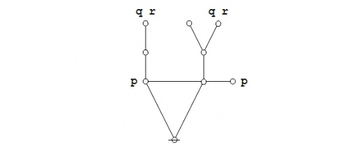
This is not only a logically equivalent DNF but exactly the same DNF expression that we obtained before, so we have established the given equation \(\texttt{(} p \texttt{(} q \texttt{))(} p \texttt{(} r \texttt{))} = \texttt{(} p \texttt{(} q r \texttt{))}.\) Incidentally, one may wish to note that this DNF expression quickly folds into the following form:

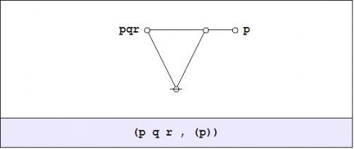
Logical Graph (P Q R , (P)).jpg (10)

This can be read to say \({}^{\backprime\backprime} \operatorname{either}~ p q r ~\operatorname{or}~ \operatorname{not}~ p {}^{\prime\prime},\) which gives us yet another equivalent for the expression \(\texttt{(} p \texttt{(} q \texttt{))(} p \texttt{(} r \texttt{))}\) and the expression \(\texttt{(} p \texttt{(} q r \texttt{))}.\) Still another way of writing the same thing would be as follows:

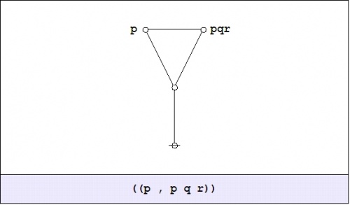
Logical Graph ((P , P Q R)).jpg (11)

In other words, \({}^{\backprime\backprime} p ~\operatorname{is~equivalent~to}~ p ~\operatorname{and}~ q ~\operatorname{and}~ r {}^{\prime\prime}.\)

One lemma that suggests itself at this point is a principle that may be canonized as the Emptiness Rule. It says that a bare lobe expression like \(\texttt{( \_, \_, \ldots )},\) with any number of places for arguments but nothing but blanks as filler, is logically tantamount to the proto-typical expression of its type, namely, the constant expression \(\texttt{(~)}\) that \(\operatorname{Ex}\) interprets as denoting the logical value \(\operatorname{false}.\) To depict the rule in graphical form, we have the continuing sequence of equations:

o-----------------------------------------------------------o
| Emptiness Rule                                            |
o-----------------------------------------------------------o
|                                                           |
|         o         o---o       o-o-o                       |
|         |          \ /         \ /                        |
|         @     =     @     =     @     =    ...            |
|                                                           |
o-----------------------------------------------------------o
(12)

Yet another rule that we'll need is the following:

o-----------------------------------------------------------o
| Indistinctness Rule                                       |
o-----------------------------------------------------------o
|                                                           |
|                   a   a       a a a                       |
|         o         o---o       o-o-o                       |
|         |          \ /         \ /                        |
|         @     =     @     =     @     =    ...            |
|                                                           |
o-----------------------------------------------------------o
(13)

This one is easy enough to derive from rules that are already known, but just for the sake of ready reference it is useful to canonize it as the Indistinctness Rule. Finally, let me introduce a rule-of-thumb that is a bit more suited to routine computation, and that serves to replace the indistinctness rule in many cases where we actually have to call on it. This is actually just a special case of the evaluation rule listed above:

o-----------------------------------------------------------o
| Evaluation Rule                                           |
o-----------------------------------------------------------o
|                                                           |
|       o                                                   |
|       |  x_2   ... x_k                                    |
|       o---o-...-o---o                                     |
|        \           /                                      |
|         \         /                                       |
|          \       /                                        |
|           \     /                                         |
|            \   /                                          |
|             \ /                       x_2 ... x_k         |
|              @              =              @              |
|                                                           |
o-----------------------------------------------------------o
|                                                           |
|     ((), x_2, ..., x_k)     =         x_2 ... x_k         |
|                                                           |
o-----------------------------------------------------------o
|            Setup      <---- | ---->      Spike            |
o-----------------------------------------------------------o
(14)

To continue with the beating of this still-kicking horse in the form of the equation \(\texttt{(} p \texttt{(} q \texttt{))(} p \texttt{(} r \texttt{))} = \texttt{(} p \texttt{(} q r \texttt{))},\) let's now take up the third way that I mentioned for examining propositional equations, even if it is literally a third way only at the very outset, almost immediately breaking up according to whether one proceeds by way of the more routine model-theoretic path or else by way of the more strategic proof-theoretic path.

Let's convert the equation between propositions:

\(\begin{matrix} \texttt{(} p \texttt{(} q \texttt{))(} p \texttt{(} r \texttt{))} & = & \texttt{(} p \texttt{(} q r \texttt{))} \end{matrix}\)

into the corresponding equational proposition:

\(\begin{matrix} \texttt{((} & \texttt{(} p \texttt{(} q \texttt{))(} p \texttt{(} r \text{))} & \texttt{,} & \texttt{(} p \texttt{(} q r \texttt{))} & \texttt{))} \end{matrix}\)

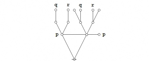
If you're like me, you'd rather see it in pictures:

Logical Graph (( (P (Q)) (P (R)) , (P (Q R)) )).jpg (15)

We may now interrogate the alleged equation for the third time, working by way of the case analysis-synthesis theorem (CAST).

Proof (P (Q)) (P (R)) = (P (Q R)) 3-00.jpg
Proof (P (Q)) (P (R)) = (P (Q R)) 3-01.jpg
Equational Inference Bar -- Cast P.jpg
Proof (P (Q)) (P (R)) = (P (Q R)) 3-02.jpg
Equational Inference Bar -- Domination.jpg
Proof (P (Q)) (P (R)) = (P (Q R)) 3-03.jpg
Equational Inference Bar -- Cancellation.jpg
Proof (P (Q)) (P (R)) = (P (Q R)) 3-04.jpg
Equational Inference Bar -- Emptiness.jpg
Proof (P (Q)) (P (R)) = (P (Q R)) 3-05.jpg
Equational Inference Bar -- Cancellation.jpg
Proof (P (Q)) (P (R)) = (P (Q R)) 3-06.jpg
Equational Inference Bar -- Cast Q.jpg
Proof (P (Q)) (P (R)) = (P (Q R)) 3-07.jpg
Equational Inference Bar -- Cancellation.jpg
Proof (P (Q)) (P (R)) = (P (Q R)) 3-08.jpg
Equational Inference Bar -- Domination.jpg
Proof (P (Q)) (P (R)) = (P (Q R)) 3-09.jpg
Equational Inference Bar -- Cancellation.jpg
Proof (P (Q)) (P (R)) = (P (Q R)) 3-10.jpg
Equational Inference Bar -- Spike.jpg
Proof (P (Q)) (P (R)) = (P (Q R)) 3-11.jpg
Equational Inference Bar -- Cancellation.jpg
Proof (P (Q)) (P (R)) = (P (Q R)) 3-12.jpg
Equational Inference Bar -- Cast R.jpg
Proof (P (Q)) (P (R)) = (P (Q R)) 3-13.jpg
Equational Inference Bar -- Cancellation.jpg
Proof (P (Q)) (P (R)) = (P (Q R)) 3-14.jpg
Equational Inference Bar -- Emptiness.jpg
Proof (P (Q)) (P (R)) = (P (Q R)) 3-15.jpg
Equational Inference Bar -- Spike.jpg
Proof (P (Q)) (P (R)) = (P (Q R)) 3-16.jpg
Equational Inference Bar -- Cancellation.jpg
Proof (P (Q)) (P (R)) = (P (Q R)) 3-17.jpg
Equational Inference Bar -- QED.jpg
(16)

And that, of course, is the DNF of a theorem.

Proof as semiosis

We have been looking at several different ways of proving one particular example of a propositional equation, and along the way we have been exemplifying the species of sign transforming process that is commonly known as a proof, more specifically, an equational proof of the propositional equation at issue. Let us now draw out these semiotic features of the business of proof and place them in relief.

Our syntactic domain \(S\!\) contains an infinite number of signs or expressions, which we may choose to view in either their text or their graphic forms, glossing over for now the many details of their parsicular correspondence.

Here are some of the expressions that we find salient enough to single out and confer an epithetic nickname on:

\(\begin{array}{lll} e_0 & = & {}^{\backprime\backprime} \texttt{(~)} {}^{\prime\prime} \\[4pt] e_1 & = & {}^{\backprime\backprime} \texttt{~} {}^{\prime\prime} \\[4pt] e_2 & = & {}^{\backprime\backprime} \texttt{(} p \texttt{~(} q \texttt{))~(} p \texttt{~(} r \texttt{))} {}^{\prime\prime} \\[4pt] e_3 & = & {}^{\backprime\backprime} \texttt{(} p \texttt{~(} q~r \texttt{))} {}^{\prime\prime} \\[4pt] e_4 & = & {}^{\backprime\backprime} \texttt{(} p~q~r \texttt{~,~(} p \texttt{))} {}^{\prime\prime} \\[4pt] e_5 & = & {}^{\backprime\backprime} \texttt{((~(} p \texttt{~(} q \texttt{))~(} p \texttt{~(} r \texttt{))~,~(} p \texttt{~(} q~r \texttt{))~))} {}^{\prime\prime} \end{array}\)

Under \(\operatorname{Ex}\) we have the following interpretations:

\(e_0 = {}^{\backprime\backprime} \texttt{(~)} {}^{\prime\prime}\) expresses the logical constant \(\operatorname{false}.\)
\(e_1 = {}^{\backprime\backprime} \texttt{~} {}^{\prime\prime}\) expresses the logical constant \(\operatorname{true}.\)
\(e_2 = {}^{\backprime\backprime} \texttt{(} p \texttt{~(} q \texttt{))~(} p \texttt{~(} r \texttt{))} {}^{\prime\prime}\) says \({}^{\backprime\backprime} \operatorname{not}~ p ~\operatorname{without}~ q,\) \(\operatorname{and~not}~ p ~\operatorname{without}~ r {}^{\prime\prime}.\)
\(e_3 = {}^{\backprime\backprime} \texttt{(} p \texttt{~(} q~r \texttt{))} {}^{\prime\prime}\) says \({}^{\backprime\backprime} \operatorname{not}~ p ~\operatorname{without}~ q ~\operatorname{and}~ r {}^{\prime\prime}.\)
\(e_4 = {}^{\backprime\backprime} \texttt{(} p~q~r \texttt{~,~(} p \texttt{))} {}^{\prime\prime}\) says \({}^{\backprime\backprime} p ~\operatorname{and}~ q ~\operatorname{and}~ r,\) \(~\operatorname{or~else~not}~ p{}^{\prime\prime}.\)
\(e_5 = {}^{\backprime\backprime} \texttt{((~(} p \texttt{~(} q \texttt{))~(} p \texttt{~(} r \texttt{))~,~(} p \texttt{~(} q~r \texttt{))~))} {}^{\prime\prime}\) says that \(e_2\!\) and \(e_3\!\) say the same thing.

We took up the Equation \(E_1\!\) that reads as follows:

\(\texttt{(} p \texttt{~(} q \texttt{))(} p \texttt{~(} r \texttt{))} = \texttt{(} p \texttt{~(} q~r \texttt{))}.\)

Each of our proofs is a finite sequence of signs, and thus, for a finite integer \(n,\!\) takes the form:

\(s_1, s_2, s_3, \ldots, s_n.\)

Proof 1 proceeded by the straightforward approach, starting with \(e_2\!\) as \(s_1\!\) and ending with \(e_3\!\) as \(s_n\!.\)

That is, Proof 1 commenced from the sign \({}^{\backprime\backprime} \texttt{(} p \texttt{~(} q \texttt{))~(} p \texttt{~(} r \texttt{))} {}^{\prime\prime}\) and ended up at the sign \({}^{\backprime\backprime} \texttt{(} p \texttt{~(} q~r \texttt{))} {}^{\prime\prime}\) by legal moves.

Proof 2 lit on by burning the candle at both ends, changing \(e_2\!\) into a normal form that reduced to \(e_4,\!\) and changing \(e_3\!\) into a normal form that also reduced to \(e_4,\!\) in this way tethering \(e_2\!\) and \(e_3\!\) to a common stake.

Filling in the details, one route went from \({}^{\backprime\backprime} \texttt{(} p \texttt{~(} q \texttt{))~(} p \texttt{~(} r \texttt{))} {}^{\prime\prime}\) to \({}^{\backprime\backprime} \texttt{(} p~q~r \texttt{~,~(} p \texttt{))} {}^{\prime\prime},\) and another went from \({}^{\backprime\backprime} \texttt{(} p \texttt{~(} q~r \texttt{))} {}^{\prime\prime}\) to \({}^{\backprime\backprime} \texttt{(} p~q~r \texttt{~,~(} p \texttt{))} {}^{\prime\prime},\) thus equating the two points of departure.

Proof 3 took the path of reflection, expressing the meta-equation between \(e_2\!\) and \(e_3\!\) in the form of the naturalized equation \(e_5,\!\) then taking \(e_5\!\) as \(s_1\!\) and exchanging it by dint of value preserving steps for \(e_1\!\) as \(s_n.\!\)

This way of proceeding went from \(e_5 = {}^{\backprime\backprime} \texttt{((~(} p \texttt{~(} q \texttt{))~(} p \texttt{~(} r \texttt{))~,~(} p \texttt{~(} q~r \texttt{))~))} {}^{\prime\prime}\) to the blank expression that \(\operatorname{Ex}\) recognizes as the value \(\operatorname{true}.\)

Computation and inference as semiosis

Equational reasoning, as distinguished from implicational reasoning, is well-evolved in mathematics today but grievously short-schrifted in contemporary logic textbooks. Consequently, it may be advisable for me to draw out and place in relief some of the more distinctive characters of equational inference that may have passed beneath the notice of a casual reading of these notes.

By way of a very preliminary orientation, let us consider the distinction between information reducing inferences and information preserving inferences. It is prudent to make make our first acquaintance with this distinction in the medium of some concrete and simple examples.

Example 1. Modus Ponens
    Information Reducing Inference
     

\(\begin{array}{l} ~ p \Rightarrow q \\ ~ p \\ \overline{~~~~~~~~~~~~~~~} \\ ~ q \end{array}\)

    Information Preserving Inference
     

\(\begin{array}{l} ~ p \Rightarrow q \\ ~ p \\ ='"`UNIQ--h-18--QINU`"'\!=\!=\!=\!=\!=\!=\!= \\ ~ p ~ q \end{array}\)

Let us examine these two types of inference in a little more detail. A rule of inference is stated in the followed form:

\(\begin{array}{l} ~ \textit{Expression~1} \\ ~ \textit{Expression~2} \\ \overline{~~~~~~~~~~~~~~~~~~~~} \\ ~ \textit{Expression~3} \end{array}\)

The expressions above the line are called premisses and the expression below the line is called a conclusion. If the rule of inference is simple enough, the proof-theoretic turnstile symbol \({}^{\backprime\backprime} \vdash {}^{\prime\prime}\) may be used to write the rule on a single line, as follows:

\(\textit{Premiss~1}, \textit{Premiss~2} ~\vdash~ \textit{Conclusion}.\)

Either way, one reads such a rule of inference in the following manner:

From   \(\textit{Expression~1}\)   and   \(\textit{Expression~2}\)   infer   \(\textit{Expression~3}.\)

Looking to Example 1, the rule of inference known as modus ponens says the following: From the premiss \(p \Rightarrow q\) and the premiss \(p\!\) one may logically infer the conclusion \(q.\!\)

Modus ponens is an illative or implicational rule. Passage through its turnstile incurs the toll of some information loss, and thus from a fact of \(q\!\) alone one cannot infer with any degree of certainty that \(p \Rightarrow q\) and \(p\!\) are the reasons why \(q\!\) happens to be true.

Further considerations along these lines may lead us to appreciate the difference between implicational rules of inference and equational rules of inference, the latter indicated by an equational line of inference or a 2-way turnstile \({}^{\backprime\backprime} \Vdash {}^{\prime\prime}.\)

Variations on a theme of transitivity

The next Example is extremely important, and for reasons that reach well beyond the level of propositional calculus as it is ordinarily conceived. But it's slightly tricky to get all of the details right, so it will be worth taking the trouble to look at it from several different angles and as it appears in diverse frames, genres, or styles of representation.

In discussing this Example, it is useful to observe that the implication relation indicated by the propositional form \(x \Rightarrow y\) is equivalent to an order relation \(x \le y\) on the boolean values \(0, 1 \in \mathbb{B},\) where \(0\!\) is taken to be less than \(1.\!\)

Example 2. Transitivity
    Information Reducing Inference
     

\(\begin{array}{l} ~ p \le q \\ ~ q \le r \\ \overline{~~~~~~~~~~~~~~~} \\ ~ p \le r \end{array}\)

    Information Preserving Inference
     

\(\begin{array}{l} ~ p \le q \\ ~ q \le r \\ ='"`UNIQ--h-20--QINU`"'\!=\!=\!=\!=\!=\!=\!= \\ ~ p \le q \le r \end{array}\)

In stating the information-preserving analogue of transitivity, I have taken advantage of a common idiom in the use of order relation symbols, one that represents their logical conjunction by way of a concatenated syntax. Thus, \(p \le q \le r\) means \(p \le q ~\operatorname{and}~ q \le r.\) The claim that this 3-adic order relation holds among the three propositions \(p, q, r\!\) is a stronger claim — conveys more information — than the claim that the 2-adic relation \(p \le r\) holds between the two propositions \(p\!\) and \(r.\!\)

To study the differences between these two versions of transitivity within what is locally a familiar context, let's view the propositional forms involved as if they were elementary cellular automaton rules, resulting in the following Table.


\(\text{Table 1.}~~\text{Composite and Compiled Order Relations}\)

\(\mathcal{L}_1\)

\(\text{Decimal}\)

\(\mathcal{L}_2\)

\(\text{Binary}\)

\(\mathcal{L}_3\)

\(\text{Vector}\)

\(\mathcal{L}_4\)

\(\text{Cactus}\)

\(\mathcal{L}_5\)

\(\text{Order}\)

  \(p\colon\!\) \(1~1~1~1~0~0~0~0\)    
  \(q\colon\!\) \(1~1~0~0~1~1~0~0\)    
  \(r\colon\!\) \(1~0~1~0~1~0~1~0\)    

\(\begin{matrix} f_{207} \\[4pt] f_{187} \\[4pt] f_{175} \\[4pt] f_{139} \end{matrix}\)

\(\begin{matrix} f_{11001111} \\[4pt] f_{10111011} \\[4pt] f_{10101111} \\[4pt] f_{10001011} \end{matrix}\)

\(\begin{matrix} 1~1~0~0~1~1~1~1 \\[4pt] 1~0~1~1~1~0~1~1 \\[4pt] 1~0~1~0~1~1~1~1 \\[4pt] 1~0~0~0~1~0~1~1 \end{matrix}\)

\(\begin{matrix} \texttt{(} p \texttt{~(} q \texttt{))} \\[4pt] \texttt{(} q \texttt{~(} r \texttt{))} \\[4pt] \texttt{(} p \texttt{~(} r \texttt{))} \\[4pt] \texttt{(} p \texttt{~(} q \texttt{))~(} q \texttt{~(} r \texttt{))} \end{matrix}\)

\(\begin{matrix} p \le q \\[4pt] q \le r \\[4pt] p \le r \\[4pt] p \le q \le r \end{matrix}\)


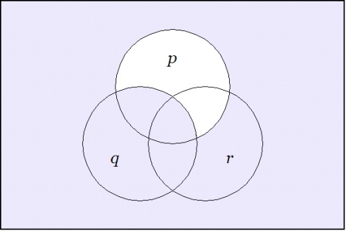
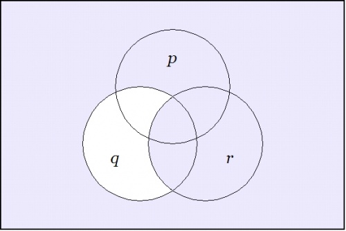
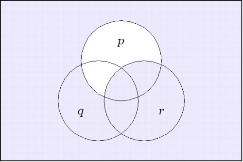
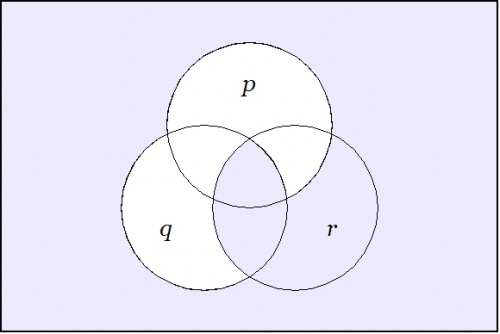
Taking up another angle of incidence by way of extra perspective, let us now reflect on the venn diagrams of our four propositions.

Venn Diagram (P (Q)).jpg (2)
\(f_{207}(p, q, r) ~=~ \texttt{(} p \texttt{~(} q \texttt{))}\)
 
Venn Diagram (Q (R)).jpg (3)
\(f_{187}(p, q, r) ~=~ \texttt{(} q \texttt{~(} r \texttt{))}\)
 
Venn Diagram (P (R)).jpg (4)
\(f_{175}(p, q, r) ~=~ \texttt{(} p \texttt{~(} r \texttt{))}\)
 
Venn Diagram (P (Q)) (Q (R)).jpg (5)
\(f_{139}(p, q, r) ~=~ \texttt{(} p \texttt{~(} q \texttt{))~(} q \texttt{~(} r \texttt{))}\)

Among other things, these images make it visually obvious that the constraint on the three boolean variables \(p, q, r\!\) that is indicated by asserting either of the forms \(\texttt{(} p \texttt{(} q \texttt{))(} q \texttt{(} r \texttt{))}\) or \(p \le q \le r\) implies a constraint on the two boolean variables \(p, r\!\) that is indicated by either of the forms \(\texttt{(} p \texttt{(} r \texttt{))}\) or \(p \le r,\) but that it imposes additional constraints on these variables that are not captured by the illative conclusion.

One way to view a proposition \(f : \mathbb{B}^k \to \mathbb{B}\) is to consider its fiber of truth, \(f^{-1}(1) \subseteq \mathbb{B}^k,\) and to regard it as a \(k\!\)-adic relation \(L \subseteq \mathbb{B}^k.\)

By way of general definition, the fiber of a function \(f : X \to Y\) at a given value \(y\!\) of its co-domain \(Y\!\) is the antecedent (also known as the inverse image or pre-image) of \(y\!\) under \(f.\!\) This is a subset, possibly empty, of the domain \(X,\!\) notated as \(f^{-1}(y) \subseteq X.\)

In particular, if \(f\!\) is a proposition \(f : X \to \mathbb{B},\) then the fiber of truth \(f^{-1}(1)\!\) is the subset of \(X\!\) that is indicated by the proposition \(f.\!\) Whenever we assert a proposition \(f : X \to \mathbb{B},\) we are saying that what it indicates is all that happens to be the case in the relevant universe of discourse \(X.\!\) Because the fiber of truth is used so often in logical contexts, it is convenient to define the more compact notation \([| f |] = f^{-1}(1).\!\)

Using this panoply of notions and notations, we may treat the fiber of truth of each proposition \(f : \mathbb{B}^3 \to \mathbb{B}\) as if it were a relational data table of the shape \(\{ (p, q, r) \} \subseteq \mathbb{B}^3,\) where the triples \((p, q, r)\!\) are bit-tuples indicated by the proposition \(f.\!\)

Thus we obtain the following four relational data tables for the propositions that we are looking at in Example 2.


\(\text{Table 6.} ~~ [| f_{207} |] ~=~ [| p \le q |]\)
\(p\!\) \(q\!\) \(r\!\)
\(0\!\) \(0\!\) \(0\!\)
\(0\!\) \(0\!\) \(1\!\)
\(0\!\) \(1\!\) \(0\!\)
\(0\!\) \(1\!\) \(1\!\)
\(1\!\) \(1\!\) \(0\!\)
\(1\!\) \(1\!\) \(1\!\)


\(\text{Table 7.} ~~ [| f_{187} |] ~=~ [| q \le r |]\)
\(p\!\) \(q\!\) \(r\!\)
\(0\!\) \(0\!\) \(0\!\)
\(0\!\) \(0\!\) \(1\!\)
\(0\!\) \(1\!\) \(1\!\)
\(1\!\) \(0\!\) \(0\!\)
\(1\!\) \(0\!\) \(1\!\)
\(1\!\) \(1\!\) \(1\!\)


\(\text{Table 8.} ~~ [| f_{175} |] ~=~ [| p \le r |]\)
\(p\!\) \(q\!\) \(r\!\)
\(0\!\) \(0\!\) \(0\!\)
\(0\!\) \(0\!\) \(1\!\)
\(0\!\) \(1\!\) \(0\!\)
\(0\!\) \(1\!\) \(1\!\)
\(1\!\) \(0\!\) \(1\!\)
\(1\!\) \(1\!\) \(1\!\)


\(\text{Table 9.} ~~ [| f_{139} |] ~=~ [| p \le q \le r |]\)
\(p\!\) \(q\!\) \(r\!\)
\(0\!\) \(0\!\) \(0\!\)
\(0\!\) \(0\!\) \(1\!\)
\(0\!\) \(1\!\) \(1\!\)
\(1\!\) \(1\!\) \(1\!\)


In the medium of these unassuming examples, we begin to see the activities of logical inference and methodical inquiry as information clarifying operations.

First, we drew a distinction between information preserving and information reducing processes and we noted the related distinction between equational and implicational inferences. I will use the acronyms EROI and IROI, respectively, for the equational and implicational analogues of the various rules of inference.

For example, we considered the brands of information fusion that are involved in a couple of standard rules of inference, taken in both their equational and their illative variants.

In particular, let us assume that we begin from a state of uncertainty about the universe of discourse \(X = \mathbb{B}^3\) that is standardly represented by a uniform distribution \(u : X \to \mathbb{B}\) such that \(u(x) = 1\!\) for all \(x\!\) in \(X,\!\) in short, by the constant proposition \(1 : X \to \mathbb{B}.\) This amounts to the maximum entropy sign state (MESS). As a measure of uncertainty, let us use either the multiplicative measure given by the cardinality of \(X,\!\) commonly notated as \(|X|,\!\) or else the additive measure given by \(\log_2 |X|.\!\) In this frame we have \(|X| = 8\!\) and \(\log_2 |X| = 3,\!\) to wit, 3 bits of doubt.

Let us now consider the various rules of inference for transitivity in the light of their performance as information-developing actions.

Transitive Law (Implicational Inference)
   

\(\begin{array}{l} ~ p \le q \\ ~ q \le r \\ \overline{~~~~~~~~~~~~~~~} \\ ~ p \le r \end{array}\)

By itself, the information \(p \le q\) would reduce our uncertainty from \(\log 8\!\) bits to \(\log 6\!\) bits.
By itself, the information \(q \le r\) would reduce our uncertainty from \(\log 8\!\) bits to \(\log 6\!\) bits.
By itself, the information \(p \le r\) would reduce our uncertainty from \(\log 8\!\) bits to \(\log 6\!\) bits.

In this situation the application of the implicational rule of inference for transitivity to the information \(p \le q\) and the information \(q \le r\) to get the information \(p \le r\) does not increase the measure of information beyond what any one of the three propositions has independently of the other two. In a sense, then, the implicational rule operates only to move the information around without changing its measure in the slightest bit.

Transitive Law (Equational Inference)
   

\(\begin{array}{l} ~ p \le q \\ ~ q \le r \\ ='"`UNIQ--h-21--QINU`"'\!=\!=\!=\!=\!=\!=\!= \\ ~ p \le q \le r \end{array}\)

The contents and the measures of information that are associated with the propositions \(p \le q\) and \(q \le r\) are the same as before.
On its own, the information \(p \le q \le r\) would reduce our uncertainty from log(8) = 3 bits to log(4) = 2 bits, a reduction of 1 bit.

These are just some of the initial observations that can be made about the dimensions of information and uncertainty in the conduct of logical inference, and there are many issues to be taken up as we get to the thick of it. In particular, we are taking propositions far too literally at the outset, reading their spots at face value, as it were, without yet considering their species character as fallible signs.

For ease of reference in the rest of this discussion, let us refer to the propositional form \(f : \mathbb{B}^3 \to \mathbb{B}\) such that \(f(p, q, r) = f_{139}(p, q, r) = \texttt{(} p \texttt{(} q \texttt{))(} q \texttt{(} r \texttt{))}\) as the syllogism map, written as \(\operatorname{syll} : \mathbb{B}^3 \to \mathbb{B},\) and let us refer to its fiber of truth \([| \operatorname{syll} |] = \operatorname{syll}^{-1}(1)\) as the syllogism relation, written as \(\operatorname{Syll} \subseteq \mathbb{B}^3.\) Table 10 shows \(\operatorname{Syll}\) as a relational dataset.


\(\text{Table 10.} ~~ \text{Syllogism Relation}\)
\(p\!\) \(q\!\) \(r\!\)
\(0\!\) \(0\!\) \(0\!\)
\(0\!\) \(0\!\) \(1\!\)
\(0\!\) \(1\!\) \(1\!\)
\(1\!\) \(1\!\) \(1\!\)


One of the first questions that we might ask about a 3-adic relation, in this case \(\operatorname{Syll},\) is whether it is determined by its 2-adic projections. I will illustrate what this means in the present case.

Table 11 repeats the relation \(\operatorname{Syll}\) in the first column, listing its 3-tuples in bit-string form, followed by the 2-adic or planar projections of \(\operatorname{Syll}\) in the next three columns. For instance, \(\operatorname{Syll}_{pq}\) is the 2-adic projection of \(\operatorname{Syll}\) on the \(pq\!\) plane that is arrived at by deleting the \(r\!\) column and counting each 2-tuple that results just one time. Likewise, \(\operatorname{Syll}_{pr}\) is obtained by deleting the \(q\!\) column and \(\operatorname{Syll}_{qr}\) is derived by deleting the \(p\!\) column, ignoring whatever duplicate pairs may result. The final row of the right three columns gives the propositions of the form \(f : \mathbb{B}^2 \to \mathbb{B}\) that indicate the 2-adic relations that result from these projections.


\(\text{Table 11.} ~~ \text{Dyadic Projections of the Syllogism Relation}\)
\(\operatorname{Syll}\) \(\operatorname{Syll}_{pq}\) \(\operatorname{Syll}_{pr}\) \(\operatorname{Syll}_{qr}\)

\(\begin{matrix} 0~0~0 \\ 0~0~1 \\ 0~1~1 \\ 1~1~1 \end{matrix}\)

\(\begin{matrix} 0~0 \\ 0~0 \\ 0~1 \\ 1~1 \end{matrix}\)

\(\begin{matrix} 0~0 \\ 0~1 \\ 0~1 \\ 1~1 \end{matrix}\)

\(\begin{matrix} 0~0 \\ 0~1 \\ 1~1 \\ 1~1 \end{matrix}\)

\(p \le q \le r\) \(\texttt{(} p \texttt{~(} q \texttt{))}\) \(\texttt{(} p \texttt{~(} r \texttt{))}\) \(\texttt{(} q \texttt{~(} r \texttt{))}\)


Let us make the simple observation that taking a projection, in our framework, deleting a column from a relational table, is like taking a derivative in differential calculus. What it means is that our attempt to return to the integral from whence the derivative was derived will in general encounter an indefinite variation on account of the circumstance that real information may have been destroyed by the derivation.

One will find that some relations can be reconstructed from various types of derivatives and projections, others cannot. The reconstuctible relations are said to be reducible to the types of reductive data in question, while the others are said to be irreducible with respect to those means.

The analogies between derivation, differentiation, implication, projection, and others sorts of information reducing operation will undergo extensive development in the remainder and sequel of the present discussion.

We were in the middle of discussing the relationships between information preserving rules of inference and information destroying rules of inference — folks of a 3-basket philosophical bent will no doubt be asking, "And what of information creating rules of inference?", but there I must wait for some signs of enlightenment, desiring not to tread on the rules of that succession.

The contrast between the information destroying and the information preserving versions of the transitive rule of inference led us to examine the relationships among several boolean functions, namely, those that qualify locally as the elementary cellular automata rules \(f_{139}, f_{175}, f_{187}, f_{207}.\!\)

The function \(f_{139} : \mathbb{B}^3 \to \mathbb{B}\) and its fiber \([| f_{139} |] \subseteq \mathbb{B}^3\) appeared to be key to many structures in this setting, and so I singled them out under the new names of \(\operatorname{syll} : \mathbb{B}^3 \to \mathbb{B}\) and \(\operatorname{Syll} \subseteq \mathbb{B}^3,\) respectively.

Managing the conceptual complexity of our considerations at this juncture put us in need of some conceptual tools that I broke off to develop in my notes on "Reductions Among Relations". The main items that we need right away from that thread are the definitions of relational projections and their inverses, the tacit extensions.

But the more I survey the problem setting the more it looks like we need better ways to bring our visual intuitions to play on the scene, and so let us next lay out some visual schemata that are designed to facilitate that.

Figure 12 shows the familiar picture of a boolean 3-cube, where the points of \(\mathbb{B}^3\) are coordinated as bit strings of length three. Looking at the functions \(f : \mathbb{B}^3 \to \mathbb{B}\) and the relations \(L \subseteq \mathbb{B}^3\) on this pattern, one views the construction of either type of object as a matter of coloring the nodes of the 3-cube with choices from a pair of colors that stipulate which points are in the relation \(L = [| f |]\!\) and which points are out of it. Bowing to common convention, we may use the color \(1\!\) for points that are in a given relation and the color \(0\!\) for points that are out of the same relation. However, it will be more convenient here to indicate the former case by writing the coordinates in the place of the node and to indicate the latter case by plotting the point as an unlabeled node "o".

o-------------------------------------------------o
|                                                 |
|                       111                       |
|                       /|\                       |
|                      / | \                      |
|                     /  |  \                     |
|                    /   |   \                    |
|                   /    |    \                   |
|                  /     |     \                  |
|                 /      |      \                 |
|               110     101     011               |
|                |\     / \     /|                |
|                | \   /   \   / |                |
|                |  \ /     \ /  |                |
|                |   \       /   |                |
|                |  / \     / \  |                |
|                | /   \   /   \ |                |
|                |/     \ /     \|                |
|               100     010     001               |
|                 \      |      /                 |
|                  \     |     /                  |
|                   \    |    /                   |
|                    \   |   /                    |
|                     \  |  /                     |
|                      \ | /                      |
|                       \|/                       |
|                       000                       |
|                                                 |
o-------------------------------------------------o
Figure 12.  Boolean 3-Cube B^3
(12)

Table 13 shows the 3-adic relation \(\operatorname{Syll} \subseteq \mathbb{B}^3\) again, and Figure 59 shows it plotted on a 3-cube template.

Table 13.  Syll c B^3
o-----------------------o
|   p       q       r   |
o-----------------------o
|   0       0       0   |
|   0       0       1   |
|   0       1       1   |
|   1       1       1   |
o-----------------------o
(13)
o-------------------------------------------------o
|                                                 |
|                       111                       |
|                       /|\                       |
|                      / | \                      |
|                     /  |  \                     |
|                    /   |   \                    |
|                   /    |    \                   |
|                  /     |     \                  |
|                 /      |      \                 |
|                o       o      011               |
|                |\     / \     /|                |
|                | \   /   \   / |                |
|                |  \ /     \ /  |                |
|                |   \       /   |                |
|                |  / \     / \  |                |
|                | /   \   /   \ |                |
|                |/     \ /     \|                |
|                o       o      001               |
|                 \      |      /                 |
|                  \     |     /                  |
|                   \    |    /                   |
|                    \   |   /                    |
|                     \  |  /                     |
|                      \ | /                      |
|                       \|/                       |
|                       000                       |
|                                                 |
o-------------------------------------------------o
Figure 14.  Triadic Relation Syll c B^3
(14)

We return once more to the plane projections of \(\operatorname{Syll} \subseteq \mathbb{B}^3.\)

Table 15.  Syll c B^3
o-----------------------o
|   p       q       r   |
o-----------------------o
|   0       0       0   |
|   0       0       1   |
|   0       1       1   |
|   1       1       1   |
o-----------------------o
(15)
Table 16.  Dyadic Projections of Syll
o-----------o o-----------o o-----------o
|  Syll_12  | |  Syll_13  | |  Syll_23  |
o-----------o o-----------o o-----------o
|   p   q   | |   p   r   | |   q   r   |
o-----------o o-----------o o-----------o
|   0   0   | |   0   0   | |   0   0   |
|   0   1   | |   0   1   | |   0   1   |
|   1   1   | |   1   1   | |   1   1   |
o-----------o o-----------o o-----------o
|  (p (q))  | |  (p (r))  | |  (q (r))  |
o-----------o o-----------o o-----------o
(16)

In showing the 2-adic projections of a 3-adic relation \(L \subseteq \mathbb{B}^3,\) I will translate the coordinates of the points in each relation to the plane of the projection, there dotting out with a dot "." the bit of the bit string that is out of place on that plane.

Figure 17 shows \(\operatorname{Syll}\) and its three 2-adic projections:

o-------------------------------------------------o
|                                                 |
|                       111                       |
|                       /|\                       |
|                      / | \                      |
|                     /  |  \                     |
|                    /   |   \                    |
|                   /    |    \                   |
|                  /     |     \                  |
|                 /      |      \                 |
|                o       o      011               |
|                |\     / \     /|                |
|                | \   /   \   / |                |
|                |  \ /     \ /  |                |
|                |   \       /   |                |
|                |  / \     / \  |                |
|                | /   \   /   \ |                |
|                |/     \ /     \|                |
|                o       o      001               |
|                 \      |      /                 |
|     11.          \     |     /          .11     |
|      |\           \    |    /           /|      |
|      | \           \   |   /           / |      |
|      |  \           \  |  /           /  |      |
|      |   \           \ | /           /   |      |
|      |    \           \|/           /    |      |
|      |     \          000          /     |      |
|      |      \                     /      |      |
|      o      01.                  o      .01     |
|       \      |                   |      /       |
|        \     |                   |     /        |
|         \    |                   |    /         |
|          \   |        1.1        |   /          |
|           \  |        / \        |  /           |
|            \ |       /   \       | /            |
|             \|      /     \      |/             |
|             00.    /       \    .00             |
|                   /         \                   |
|                  /           \                  |
|                 /             \                 |
|                o              0.1               |
|                 \             /                 |
|                  \           /                  |
|                   \         /                   |
|                    \       /                    |
|                     \     /                     |
|                      \   /                      |
|                       \ /                       |
|                       0.0                       |
|                                                 |
o-------------------------------------------------o
Figure 17.  Syll c B^3 and its Dyadic Projections
(17)

We now compute the tacit extensions of the 2-adic projections of \(\operatorname{Syll},\) alias \(f_{139},\!\) and this makes manifest its relationship to the other functions and fibers, namely, \(f_{175}, f_{187}, f_{207}.\!\)

Table 18.  Syll c B^3
o-----------------------o
|   p       q       r   |
o-----------------------o
|   0       0       0   |
|   0       0       1   |
|   0       1       1   |
|   1       1       1   |
o-----------------------o
(18)
Table 19.  Dyadic Projections of Syll
o-----------o o-----------o o-----------o
|  Syll_12  | |  Syll_13  | |  Syll_23  |
o-----------o o-----------o o-----------o
|   p   q   | |   p   r   | |   q   r   |
o-----------o o-----------o o-----------o
|   0   0   | |   0   0   | |   0   0   |
|   0   1   | |   0   1   | |   0   1   |
|   1   1   | |   1   1   | |   1   1   |
o-----------o o-----------o o-----------o
|  (p (q))  | |  (p (r))  | |  (q (r))  |
o-----------o o-----------o o-----------o
(19)
Table 20.  Tacit Extensions of Projections of Syll
o---------------o o---------------o o---------------o
|  te(Syll_12)  | |  te(Syll_13)  | |  te(Syll_23)  |
o---------------o o---------------o o---------------o
|   p   q   r   | |   p   q   r   | |   p   q   r   |
o---------------o o---------------o o---------------o
|   0   0   0   | |   0   0   0   | |   0   0   0   |
|   0   0   1   | |   0   1   0   | |   1   0   0   |
|   0   1   0   | |   0   0   1   | |   0   0   1   |
|   0   1   1   | |   0   1   1   | |   1   0   1   |
|   1   1   0   | |   1   0   1   | |   0   1   1   |
|   1   1   1   | |   1   1   1   | |   1   1   1   |
o---------------o o---------------o o---------------o
| [| (p (q)) |] | | [| (p (r)) |] | | [| (q (r)) |] |
o---------------o o---------------o o---------------o
| [|  f_207  |] | | [|  f_175  |] | | [|  f_187  |] |
o---------------o o---------------o o---------------o
(20)
o-------------------------------------------------o
|                                                 |
|                       111                       |
|                       /|\                       |
|                      / | \                      |
|                     /  |  \                     |
|                    /   |   \                    |
|                   /    |    \                   |
|                  /     |     \                  |
|                 /      |      \                 |
|               110      o      011               |
|                |\     / \     /|                |
|                | \   /   \   / |                |
|                |  \ /     \ /  |                |
|                |   \       /   |                |
|                |  / \     / \  |                |
|                | /   \   /   \ |                |
|                |/     \ /     \|                |
|                o      010     001               |
|                 \      |      /                 |
|     11.          \     |     /                  |
|      |\           \    |    /                   |
|      | \           \   |   /                    |
|      |  \           \  |  /                     |
|      |   \           \ | /                      |
|      |    \           \|/                       |
|      |     \          000                       |
|      |      \                                   |
|      o      01.                                 |
|       \      |                                  |
|        \     |                                  |
|         \    |                                  |
|          \   |                                  |
|           \  |                                  |
|            \ |                                  |
|             \|                                  |
|             00.                                 |
|                                                 |
o-------------------------------------------------o
Figure 21.  Tacit Extension te_12_3 (Syll_12)
(21)
o-------------------------------------------------o
|                                                 |
|                       111                       |
|                       /|\                       |
|                      / | \                      |
|                     /  |  \                     |
|                    /   |   \                    |
|                   /    |    \                   |
|                  /     |     \                  |
|                 /      |      \                 |
|                o      101     011               |
|                |\     / \     /|                |
|                | \   /   \   / |                |
|                |  \ /     \ /  |                |
|                |   \       /   |                |
|                |  / \     / \  |                |
|                | /   \   /   \ |                |
|                |/     \ /     \|                |
|                o      010     001               |
|                 \      |      /                 |
|                  \     |     /                  |
|                   \    |    /                   |
|                    \   |   /                    |
|                     \  |  /                     |
|                      \ | /                      |
|                       \|/                       |
|                       000                       |
|                                                 |
|                                                 |
|                       1.1                       |
|                       / \                       |
|                      /   \                      |
|                     /     \                     |
|                    /       \                    |
|                   /         \                   |
|                  /           \                  |
|                 /             \                 |
|                o              0.1               |
|                 \             /                 |
|                  \           /                  |
|                   \         /                   |
|                    \       /                    |
|                     \     /                     |
|                      \   /                      |
|                       \ /                       |
|                       0.0                       |
|                                                 |
o-------------------------------------------------o
Figure 22.  Tacit Extension te_13_2 (Syll_13)
(22)
o-------------------------------------------------o
|                                                 |
|                       111                       |
|                       /|\                       |
|                      / | \                      |
|                     /  |  \                     |
|                    /   |   \                    |
|                   /    |    \                   |
|                  /     |     \                  |
|                 /      |      \                 |
|                o      101     011               |
|                |\     / \     /|                |
|                | \   /   \   / |                |
|                |  \ /     \ /  |                |
|                |   \       /   |                |
|                |  / \     / \  |                |
|                | /   \   /   \ |                |
|                |/     \ /     \|                |
|               100      o      001               |
|                 \      |      /                 |
|                  \     |     /          .11     |
|                   \    |    /           /|      |
|                    \   |   /           / |      |
|                     \  |  /           /  |      |
|                      \ | /           /   |      |
|                       \|/           /    |      |
|                       000          /     |      |
|                                   /      |      |
|                                  o      .01     |
|                                  |      /       |
|                                  |     /        |
|                                  |    /         |
|                                  |   /          |
|                                  |  /           |
|                                  | /            |
|                                  |/             |
|                                 .00             |
|                                                 |
o-------------------------------------------------o
Figure 23.  Tacit Extension te_23_1 (Syll_23)
(23)

The reader may wish to contemplate Figure 24 and use it to verify the following two facts:

\(\begin{array}{lcc} \operatorname{Syll} & = & \operatorname{te}(\operatorname{Syll}_{12}) \cap \operatorname{te}(\operatorname{Syll}_{23}) \\[6pt] \operatorname{Syll}_{13} & = & \operatorname{Syll}_{12} \circ \operatorname{Syll}_{23} \end{array}\)

o-------------------------------------------------o
|                                                 |
|                        *                        |
|                       /|\                       |
|                      / | \                      |
|                     /  |  \                     |
|                    /   |   \                    |
|                   /    |    \                   |
|                  /     |     \                  |
|                 /      |      \                 |
|                o       o       *                |
|               /|\     / \     /|\               |
|              / | \   /   \   / | \              |
|             /  |  \ /     \ /  |  \             |
|            /   |   \       /   |   \            |
|           /    |  / \     / \  |    \           |
|          /     | /   \   /   \ |     \          |
|         /      |/     \ /     \|      \         |
|        /       o       o       *       \        |
|       /         \     /|      / \       \       |
|      *           \   / |     /   \       *      |
|      |\           \ /  |    /     \     /|      |
|      | \           /   |   /       \   / |      |
|      |  \         / \  |  /         \ /  |      |
|      |   \       /   \ | /           /   |      |
|      |    \     /     \|/           / \  |      |
|      |     \   /       *           /   \ |      |
|      |      \ /       / \         /     \|      |
|      o       *       /   \       o       *      |
|       \      |      /     \      |      /       |
|        \     |     /       \     |     /        |
|         \    |    /         \    |    /         |
|          \   |   /     *     \   |   /          |
|           \  |  /     / \     \  |  /           |
|            \ | /     /   \     \ | /            |
|             \|/     /     \     \|/             |
|              *     /       \     *              |
|                   /         \                   |
|                  /           \                  |
|                 /             \                 |
|                o               *                |
|                 \             /                 |
|                  \           /                  |
|                   \         /                   |
|                    \       /                    |
|                     \     /                     |
|                      \   /                      |
|                       \ /                       |
|                        *                        |
|                                                 |
o-------------------------------------------------o
Figure 24.  Syll = te(Syll_12) |^| te(Syll_23)
(24)

I don't know about you, but I am still puzzled by all of thus stuff, that is to say, by the entanglements of composition and projection and their relationship to the information processing properties of logical inference rules. What I lack is a single picture that could show me all of the pieces and make the pattern of their informational relationships clear.

In accord with my experimental way, I will stick with the case of transitive inference until I have pinned it down thoroughly, but of course the real interest is much more general than that.

At first sight, the relationships seem easy enough to write out. Figure 25 shows how the various logical expressions are related to each other: The expressions \({}^{\backprime\backprime} \texttt{(} p \texttt{~(} q \texttt{))} {}^{\prime\prime}\) and \({}^{\backprime\backprime} \texttt{(} q \texttt{~(} r \texttt{))} {}^{\prime\prime}\) are conjoined in a purely syntactic fashion — much in the way that one might compile a theory from axioms without knowing what either the theory or the axioms were about — and the best way to sum up the state of information implicit in taking them together is just the expression \({}^{\backprime\backprime} \texttt{(} p \texttt{~(} q \texttt{))~(} q \texttt{~(} r \texttt{))}{}^{\prime\prime}\) that would the canonical result of an equational or reversible rule of inference. From that equational inference, one might arrive at the implicational inference \({}^{\backprime\backprime} \texttt{(} p \texttt{~(} r \texttt{))} {}^{\prime\prime}\) by the most conventional implication.

o-------------------o         o-------------------o
|                   |         |                   |
|         q         |         |         r         |
|         o         |         |         o         |
|         |         |         |         |         |
|       p o         |         |       q o         |
|         |         |         |         |         |
|         @         |         |         @         |
|                   |         |                   |
o-------------------o         o-------------------o
|      (p (q))      |         |      (q (r))      |
o-------------------o         o-------------------o
|       f_207       |         |       f_187       |
o---------o---------o         o---------o---------o
           \                           /           
            \       Conjunction       /            
             \                       /             
              v                     v              
               o-------------------o               
               |                   |               
               |                   |               
               |                   |               
               |       q   r       |               
               |       o   o       |               
               |       |   |       |               
               |     p o   o q     |               
               |        \ /        |               
               |         @         |               
               |                   |               
               o-------------------o               
               |  (p (q)) (q (r))  |               
               o-------------------o               
               |       f_139       |               
               o---------o---------o               
                         |                         
                    Implication                    
                         |                         
                         v                         
               o---------o---------o               
               |                   |               
               |         r         |               
               |         o         |               
               |         |         |               
               |       p o         |               
               |         |         |               
               |         @         |               
               |                   |               
               o-------------------o               
               |      (p (r))      |               
               o-------------------o               
               |       f_175       |               
               o-------------------o               
                                                   
Figure 25.  Expressive Aspects of Transitive Inference

Most of the customary names for this type of process have turned out to have misleading connotations, and so I will experiment with calling it the expressive aspect of the various rules for transitive inference, simply to emphasize the fact that rules can be given for it that operate solely on signs and expressions, without necessarily needing to look at the objects that are denoted by these signs and expressions.

In the way of many experiments, the word expressive does not seem to work for what I wanted to say here, since we too often use it to suggest something that expresses an object or a purpose, and I wanted it to imply what is purely a matter of expression, shorn of consideration for anything objective. Aside from coining a word like ennotative, some other options would be connotative, hermeneutic, semiotic, syntactic — each of which works in some range of interpretation but fails in others. Let's try formulaic.

Despite how simple the formulaic aspects of transitive inference might appear on the surface, there are problems that wait for us just beneath the syntactic surface, as we quickly discover if we turn to considering the kinds of objects, abstract and concrete, that these formulas are meant to denote, and all the more so if we try to do this in a context of computational implementations, where the "interpreters" to be addressed take nothing on faith. Thus we engage the denotative semantics or the model theory of these extremely simple programs that we call propositions.

Figure 26 is an attempt to outline the model-theoretic relationships that are involved in our study of transitive inference. A couple of alternative notations are introduced in this Table:

The forms \(X:Y:Z\!\) and \(x:y:z\!\) are used as alternative notations for the cartesian product \(X \times Y \times Z\) and the tuple \((x, y, z),\!\) respectively.
In situations where we have products like \(X:Y:Z\!\) with \(X = Y = Z = \mathbb{B},\) and relations like \(L \subseteq X:Y,\)   \(M \subseteq X:Z,\)   \(N \subseteq Y:Z,\) the forms \(L \subseteq \mathbb{B}:\mathbb{B}:-,\)   \(M \subseteq \mathbb{B}:-:\mathbb{B},\)   \(N \subseteq -:\mathbb{B}:\mathbb{B}\) are used to remind us that we are considering particular ways of situating \(L, M, N\!\) within the product space \(X:Y:Z.\!\)
o-------------------o         o-------------------o
|                   |         |                   |
|       0:0:0       |         |       0:0:0       |
|       0:0:1       |         |       0:0:1       |
|       0:1:0       |         |       0:1:1       |
|       0:1:1       |         |       1:0:0       |
|       1:1:0       |         |       1:0:1       |
|       1:1:1       |         |       1:1:1       |
|                   |         |                   |
o-------------------o         o-------------------o
|te(Syll_12) c B:B:B|         |te(Syll_23) c B:B:B|
o-------------------o         o-------------------o
|    [| f_207 |]    |         |    [| f_187 |]    |
o----o---------o----o         o----o---------o----o
     ^          \                 /          ^     
     |           \ Intersection  /           |     
     |            \             /            |     
     |             v           v             |     
     |         o-------------------o         |     
     |         |                   |         |     
     |         |       0:0:0       |         |     
     |         |       0:0:1       |         |     
     |         |       0:1:1       |         |     
     |         |       1:1:1       |         |     
     |         |                   |         |     
     |         o-------------------o         |     
     |         |    Syll c B:B:B   |         |     
     |         o-------------------o         |     
     |         |    [| f_139 |]    |         |     
     |         o---------o---------o         |     
     |                   |                   |     
     |              Projection               |     
     |                   |                   |     
     |                   v                   |     
     |         o---------o---------o         |     
     |         |                   |         |     
     |         |        0:0        |         |     
     |         |        0:1        |         |     
     |         |        1:1        |         |     
     |         |                   |         |     
     |         o-------------------o         |     
     |         |  Syll_13 c B:~:B  |         |     
     |         o-------------------o         |     
     |         |   [| (p (r)) |]   |         |     
     |         o----o---------o----o         |     
     |             ^           ^             |     
     |            /             \            |     
     |           /  Composition  \           |     
     |          /                 \          |     
o----o---------o----o         o----o---------o----o
|                   |         |                   |
|        0:0        |         |        0:0        |
|        0:1        |         |        0:1        |
|        1:1        |         |        1:1        |
|                   |         |                   |
o-------------------o         o-------------------o
|  Syll_12 c B:B:~  |         |  Syll_23 c ~:B:B  |
o-------------------o         o-------------------o
|   [| (p (q)) |]   |         |   [| (q (r)) |]   |
o---------o---------o         o---------o---------o
                                                   
Figure 26.  Denotative Aspects of Transitive Inference

A piece of syntax like \({}^{\backprime\backprime} \texttt{(} p \texttt{(} q \texttt{))} {}^{\prime\prime}\) or \({}^{\backprime\backprime} p \Rightarrow q {}^{\prime\prime}\) is an abstract description, and abstraction is a process that loses information about the objects described. So when we go to reverse the abstraction, as we do when we look for models of that description, there is a degree of indefiniteness that comes into play.

For example, the proposition \(\texttt{(} p \texttt{(} q \texttt{))}\) is typically assigned the functional type \(\mathbb{B}^2 \to \mathbb{B},\) but that is only its canonical or its minimal abstract type. No sooner do we use it in a context that invokes additional variables, as we do when we next consider the proposition \(\texttt{(} q \texttt{(} r \texttt{))},\) than its type is tacitly adjusted to fit the new context, for instance, acquiring the extended type \(\mathbb{B}^3 \to \mathbb{B}.\) This is one of those things that most people eventually learn to do without blinking an eye, that is to say, unreflectively, and this is precisely what makes the same facility so much trouble to implement properly in computational form.

Both the fibering operation, that takes us from the function \(\texttt{(} p \texttt{(} q \texttt{))}\) to the relation \([| \texttt{(} p \texttt{(} q \texttt{))} |],\) and the tacit extension operation, that takes us from the relation \([| \texttt{(} p \texttt{(} q \texttt{))} |] \subseteq \mathbb{B}:\mathbb{B}\) to the relation \([| q_{207} |] \subseteq \mathbb{B}:\mathbb{B}:\mathbb{B},\) have this same character of abstraction-undoing or modelling operations that require us to re-interpret the same pieces of syntax under different types. This accounts for a large part of the apparent ambiguities.

Up till now I've concentrated mostly on the abstract types of domains and propositions, things like \(\mathbb{B}^k\) and \(\mathbb{B}^k \to \mathbb{B},\) respectively. This is a little like trying to do physics all in dimensionless quantities without keeping track of the qualitative physical units. So much abstraction has its obvious limits, not to mention its hidden dangers.

To remedy this situation I will start to introduce the concrete types of domains and propositions, once again as they pertain to our current collection of examples.

We have been using the lower case letters \(p, q, r\!\) for the basic propositions of abstract type \(\mathbb{B}^3 \to \mathbb{B}\) and the upper case letters \(P, Q, R\!\) for the basic regions of the universe of discourse where \(p, q, r,\!\) respectively, hold true.

The set of signs \(\mathcal{X} = \{ {}^{\backprime\backprime} p {}^{\prime\prime}, {}^{\backprime\backprime} q {}^{\prime\prime}, {}^{\backprime\backprime} r {}^{\prime\prime} \}\) is the alphabet for the universe of discourse that is notated as \(X^\circ = [\mathcal{X}] = [p, q, r],\) already getting sloppy about quotation marks to single out the signs.

The universe \(X^\circ\) is composed of two different spaces of objects. The first is the space of positions \(X = \langle p, q, r \rangle = \{ (p, q, r) \}.\) The second is the space of propositions \(X^\uparrow = (X \to \mathbb{B}).\)

Let us make the following definitions:

\(\begin{matrix} P^\ddagger & = & X_p & = & \{ \texttt{(} p \texttt{)}, p \}, \\[4pt] Q^\ddagger & = & X_q & = & \{ \texttt{(} q \texttt{)}, q \}, \\[4pt] R^\ddagger & = & X_r & = & \{ \texttt{(} r \texttt{)}, r \}. \end{matrix}\)

These are three sets of two abstract signs each, altogether staking out the qualitative dimensions of the universe of discourse \(X^\circ\).

Given this framework, the concrete type of the space \(X\!\) is \(P^\ddagger \times Q^\ddagger \times R^\ddagger ~\cong~ \mathbb{B}^3\) and the concrete type of each proposition in \(X^\uparrow = (X \to \mathbb{B})\) is \(P^\ddagger \times Q^\ddagger \times R^\ddagger \to \mathbb{B}.\) Given the length of the type markers, we will often omit the cartesian product symbols and write just \(P^\ddagger Q^\ddagger R^\ddagger.\)

An abstract reference to a point of \(X\!\) is a triple in \(\mathbb{B}^3.\) A concrete reference to a point of \(X\!\) is a conjunction of signs from the dimensions \(P^\ddagger, Q^\ddagger, R^\ddagger,\) picking exactly one sign from each dimension.

To illustrate the use of concrete coordinates for points and concrete types for spaces and propositions, Figure 27 translates the contents of Figure 26 into the new language.

o-------------------o         o-------------------o
|                   |         |                   |
|     (p)(q)(r)     |         |     (p)(q)(r)     |
|     (p)(q) r      |         |     (p)(q) r      |
|     (p) q (r)     |         |     (p) q  r      |
|     (p) q  r      |         |      p (q)(r)     |
|      p  q (r)     |         |      p (q) r      |
|      p  q  r      |         |      p  q  r      |
|                   |         |                   |
o-------------------o         o-------------------o
|TE(Syll_12) c B:B:B|         |TE(Syll_23) c B:B:B|
o-------------------o         o-------------------o
|    [| f_207 |]    |         |    [| f_187 |]    |
o----o---------o----o         o----o---------o----o
     ^          \                 /          ^     
     |           \ Intersection  /           |     
     |            \             /            |     
     |             v           v             |     
     |         o-------------------o         |     
     |         |                   |         |     
     |         |     (p)(q)(r)     |         |     
     |         |     (p)(q) r      |         |     
     |         |     (p) q  r      |         |     
     |         |      p  q  r      |         |     
     |         |                   |         |     
     |         o-------------------o         |     
     |         |  Syll c P‡ Q‡ R‡  |         |     
     |         o-------------------o         |     
     |         |    [| f_139 |]    |         |     
     |         o---------o---------o         |     
     |                   |                   |     
     |              Projection               |     
     |                   |                   |     
     |                   v                   |     
     |         o---------o---------o         |     
     |         |                   |         |     
     |         |      (p) (r)      |         |     
     |         |      (p)  r       |         |     
     |         |       p   r       |         |     
     |         |                   |         |     
     |         o-------------------o         |     
     |         |  Syll_13 c P‡ R‡  |         |     
     |         o-------------------o         |     
     |         |   [| (p (r)) |]   |         |     
     |         o----o---------o----o         |     
     |             ^           ^             |     
     |            /             \            |     
     |           /  Composition  \           |     
     |          /                 \          |     
o----o---------o----o         o----o---------o----o
|                   |         |                   |
|      (p) (q)      |         |      (q) (r)      |
|      (p)  q       |         |      (q)  r       |
|       p   q       |         |       q   r       |
|                   |         |                   |
o-------------------o         o-------------------o
|  Syll_12 c P‡ Q‡  |         |  Syll_23 c Q‡ R‡  |
o-------------------o         o-------------------o
|   [| (p (q)) |]   |         |   [| (q (r)) |]   |
o---------o---------o         o---------o---------o
                                                    
Figure 27.  Denotative Aspects of Transitive Inference

References

  • Leibniz, G.W. (1679–1686 ?), "Addenda to the Specimen of the Universal Calculus", pp. 40–46 in Parkinson, G.H.R. (ed.), Leibniz : Logical Papers, Oxford University Press, London, UK, 1966. (Cf. Gerhardt, 7, p. 223).
  • Peirce, C.S. (1981–), Writings of Charles S. Peirce: A Chronological Edition, Peirce Edition Project (eds.), Indiana University Press, Bloomington and Indianoplis, IN. Cited as CE volume, page.
  • Peirce, C.S. (1885), "On the Algebra of Logic: A Contribution to the Philosophy of Notation", American Journal of Mathematics 7 (1885), 180–202. Reprinted as CP 3.359–403 and CE 5, 162–190.
  • Peirce, C.S. (c. 1886), "Qualitative Logic", MS 736. Published as pp. 101–115 in Carolyn Eisele (ed., 1976), The New Elements of Mathematics by Charles S. Peirce, Volume 4, Mathematical Philosophy, Mouton, The Hague.
  • Peirce, C.S. (1886 a), "Qualitative Logic", MS 582. Published as pp. 323–371 in Writings of Charles S. Peirce: A Chronological Edition, Volume 5, 1884–1886, Peirce Edition Project (eds.), Indiana University Press, Bloomington, IN, 1993.
  • Peirce, C.S. (1886 b), "The Logic of Relatives: Qualitative and Quantitative", MS 584. Published as pp. 372–378 in Writings of Charles S. Peirce: A Chronological Edition, Volume 5, 1884–1886, Peirce Edition Project (eds.), Indiana University Press, Bloomington, IN, 1993.

See also

Related essays and projects

Related concepts and topics

Template:Col-breakTemplate:Col-breakTemplate:Col-breakTemplate:Col-end

External links

Document history

Standard Upper Ontology (Mar–Apr 2001)

  1. http://suo.ieee.org/email/msg04187.html
  2. http://suo.ieee.org/email/msg04305.html
  3. http://suo.ieee.org/email/msg04413.html
  4. http://suo.ieee.org/email/msg04419.html
  5. http://suo.ieee.org/email/msg04422.html
  6. http://suo.ieee.org/email/msg04423.html
  7. http://suo.ieee.org/email/msg04432.html
  8. http://suo.ieee.org/email/msg04454.html
  9. http://suo.ieee.org/email/msg04455.html
  10. http://suo.ieee.org/email/msg04476.html
  11. http://suo.ieee.org/email/msg04510.html
  12. http://suo.ieee.org/email/msg04517.html
  13. http://suo.ieee.org/email/msg04525.html
  14. http://suo.ieee.org/email/msg04533.html
  15. http://suo.ieee.org/email/msg04536.html
  16. http://suo.ieee.org/email/msg04542.html
  17. http://suo.ieee.org/email/msg04546.html

Ontology List (Mar–Apr 2001)

  1. http://suo.ieee.org/ontology/msg01779.html
  2. http://suo.ieee.org/ontology/msg01897.html
  3. http://suo.ieee.org/ontology/msg02005.html
  4. http://suo.ieee.org/ontology/msg02011.html
  5. http://suo.ieee.org/ontology/msg02014.html
  6. http://suo.ieee.org/ontology/msg02015.html
  7. http://suo.ieee.org/ontology/msg02024.html
  8. http://suo.ieee.org/ontology/msg02046.html
  9. http://suo.ieee.org/ontology/msg02047.html
  10. http://suo.ieee.org/ontology/msg02068.html
  11. http://suo.ieee.org/ontology/msg02102.html
  12. http://suo.ieee.org/ontology/msg02109.html
  13. http://suo.ieee.org/ontology/msg02117.html
  14. http://suo.ieee.org/ontology/msg02125.html
  15. http://suo.ieee.org/ontology/msg02128.html
  16. http://suo.ieee.org/ontology/msg02134.html
  17. http://suo.ieee.org/ontology/msg02138.html

Arisbe List (Feb 2003)

  1. http://stderr.org/pipermail/arisbe/2003-February/001541.html
  2. http://stderr.org/pipermail/arisbe/2003-February/001542.html
  3. http://stderr.org/pipermail/arisbe/2003-February/001543.html
  4. http://stderr.org/pipermail/arisbe/2003-February/001544.html
  5. http://stderr.org/pipermail/arisbe/2003-February/001545.html
  6. http://stderr.org/pipermail/arisbe/2003-February/001546.html
  7. http://stderr.org/pipermail/arisbe/2003-February/001547.html
  8. http://stderr.org/pipermail/arisbe/2003-February/001548.html
  9. http://stderr.org/pipermail/arisbe/2003-February/001549.html
  10. http://stderr.org/pipermail/arisbe/2003-February/001550.html
  11. http://stderr.org/pipermail/arisbe/2003-February/001552.html
  12. http://stderr.org/pipermail/arisbe/2003-February/001553.html
  13. http://stderr.org/pipermail/arisbe/2003-February/001554.html
  14. http://stderr.org/pipermail/arisbe/2003-February/001555.html
  15. http://stderr.org/pipermail/arisbe/2003-February/001557.html
  16. http://stderr.org/pipermail/arisbe/2003-February/001559.html

Ontology List (Feb 2003)

  1. http://suo.ieee.org/ontology/msg04522.html
  2. http://suo.ieee.org/ontology/msg04523.html
  3. http://suo.ieee.org/ontology/msg04524.html
  4. http://suo.ieee.org/ontology/msg04525.html
  5. http://suo.ieee.org/ontology/msg04526.html
  6. http://suo.ieee.org/ontology/msg04527.html
  7. http://suo.ieee.org/ontology/msg04528.html
  8. http://suo.ieee.org/ontology/msg04529.html
  9. http://suo.ieee.org/ontology/msg04530.html
  10. http://suo.ieee.org/ontology/msg04531.html
  11. http://suo.ieee.org/ontology/msg04532.html
  12. http://suo.ieee.org/ontology/msg04533.html
  13. http://suo.ieee.org/ontology/msg04534.html
  14. http://suo.ieee.org/ontology/msg04536.html
  15. http://suo.ieee.org/ontology/msg04537.html
  16. http://suo.ieee.org/ontology/msg04538.html

Inquiry List (Mar 2003)

  1. http://stderr.org/pipermail/inquiry/2003-March/000126.html
  2. http://stderr.org/pipermail/inquiry/2003-March/000127.html
  3. http://stderr.org/pipermail/inquiry/2003-March/000128.html
  4. http://stderr.org/pipermail/inquiry/2003-March/000129.html
  5. http://stderr.org/pipermail/inquiry/2003-March/000130.html
  6. http://stderr.org/pipermail/inquiry/2003-March/000131.html
  7. http://stderr.org/pipermail/inquiry/2003-March/000132.html
  8. http://stderr.org/pipermail/inquiry/2003-March/000133.html
  9. http://stderr.org/pipermail/inquiry/2003-March/000134.html
  10. http://stderr.org/pipermail/inquiry/2003-March/000135.html
  11. http://stderr.org/pipermail/inquiry/2003-March/000136.html
  12. http://stderr.org/pipermail/inquiry/2003-March/000137.html
  13. http://stderr.org/pipermail/inquiry/2003-March/000138.html
  14. http://stderr.org/pipermail/inquiry/2003-March/000139.html
  15. http://stderr.org/pipermail/inquiry/2003-March/000140.html
  16. http://stderr.org/pipermail/inquiry/2003-March/000141.html
  17. http://stderr.org/pipermail/inquiry/2003-March/000142.html

NKS Forum (Apr–May 2004)

  1. http://forum.wolframscience.com/showthread.php?postid=950#post950
  2. http://forum.wolframscience.com/showthread.php?postid=952#post952
  3. http://forum.wolframscience.com/showthread.php?postid=953#post953
  4. http://forum.wolframscience.com/showthread.php?postid=954#post954
  5. http://forum.wolframscience.com/showthread.php?postid=957#post957
  6. http://forum.wolframscience.com/showthread.php?postid=958#post958
  7. http://forum.wolframscience.com/showthread.php?postid=959#post959
  8. http://forum.wolframscience.com/showthread.php?postid=961#post961
  9. http://forum.wolframscience.com/showthread.php?postid=962#post962
  10. http://forum.wolframscience.com/showthread.php?postid=964#post964
  11. http://forum.wolframscience.com/showthread.php?postid=965#post965
  12. http://forum.wolframscience.com/showthread.php?postid=967#post967
  13. http://forum.wolframscience.com/showthread.php?postid=968#post968
  14. http://forum.wolframscience.com/showthread.php?postid=973#post973
  15. http://forum.wolframscience.com/showthread.php?postid=976#post976
  16. http://forum.wolframscience.com/showthread.php?postid=977#post977
  17. http://forum.wolframscience.com/showthread.php?postid=981#post981
  18. http://forum.wolframscience.com/showthread.php?postid=988#post988
  19. http://forum.wolframscience.com/showthread.php?postid=990#post990
  20. http://forum.wolframscience.com/showthread.php?postid=994#post994
  21. http://forum.wolframscience.com/showthread.php?postid=1003#post1003
  22. http://forum.wolframscience.com/showthread.php?postid=1005#post1005
  23. http://forum.wolframscience.com/showthread.php?postid=1015#post1015
  24. http://forum.wolframscience.com/showthread.php?postid=1022#post1022
  25. http://forum.wolframscience.com/showthread.php?postid=1025#post1025
  26. http://forum.wolframscience.com/showthread.php?postid=1031#post1031
  27. http://forum.wolframscience.com/showthread.php?postid=1220#post1220
  28. http://forum.wolframscience.com/showthread.php?postid=1224#post1224
  29. http://forum.wolframscience.com/showthread.php?postid=1227#post1227
  30. http://forum.wolframscience.com/showthread.php?postid=1228#post1228
  31. http://forum.wolframscience.com/showthread.php?postid=1232#post1232
  32. http://forum.wolframscience.com/showthread.php?postid=1249#post1249
  33. http://forum.wolframscience.com/showthread.php?postid=1262#post1262
  34. http://forum.wolframscience.com/showthread.php?postid=1265#post1265
  35. http://forum.wolframscience.com/showthread.php?postid=1273#post1273

Inquiry List (2004–2006)

  1. http://stderr.org/pipermail/inquiry/2004-April/001341.html
  2. http://stderr.org/pipermail/inquiry/2004-April/001342.html
  3. http://stderr.org/pipermail/inquiry/2004-April/001343.html
  4. http://stderr.org/pipermail/inquiry/2004-April/001344.html
  5. http://stderr.org/pipermail/inquiry/2004-April/001345.html
  6. http://stderr.org/pipermail/inquiry/2004-April/001346.html
  7. http://stderr.org/pipermail/inquiry/2004-April/001347.html
  8. http://stderr.org/pipermail/inquiry/2004-April/001348.html
  9. http://stderr.org/pipermail/inquiry/2004-April/001349.html
  10. http://stderr.org/pipermail/inquiry/2004-April/001350.html
  11. http://stderr.org/pipermail/inquiry/2004-April/001351.html
  12. http://stderr.org/pipermail/inquiry/2004-April/001352.html
  13. http://stderr.org/pipermail/inquiry/2004-April/001353.html
  14. http://stderr.org/pipermail/inquiry/2004-April/001354.html
  15. http://stderr.org/pipermail/inquiry/2004-April/001355.html
  16. http://stderr.org/pipermail/inquiry/2004-April/001356.html
  17. http://stderr.org/pipermail/inquiry/2004-April/001357.html
  18. http://stderr.org/pipermail/inquiry/2004-April/001358.html
  19. http://stderr.org/pipermail/inquiry/2004-April/001359.html
  20. http://stderr.org/pipermail/inquiry/2004-April/001360.html
  21. http://stderr.org/pipermail/inquiry/2004-April/001361.html
  22. http://stderr.org/pipermail/inquiry/2004-April/001362.html
  23. http://stderr.org/pipermail/inquiry/2004-April/001363.html
  24. http://stderr.org/pipermail/inquiry/2004-April/001364.html
  25. http://stderr.org/pipermail/inquiry/2004-April/001365.html
  26. http://stderr.org/pipermail/inquiry/2004-April/001366.html
  27. http://stderr.org/pipermail/inquiry/2004-April/001389.html
  28. http://stderr.org/pipermail/inquiry/2004-April/001390.html
  29. http://stderr.org/pipermail/inquiry/2004-May/001391.html
  30. http://stderr.org/pipermail/inquiry/2004-May/001392.html
  31. http://stderr.org/pipermail/inquiry/2004-May/001393.html
  32. http://stderr.org/pipermail/inquiry/2004-May/001394.html
  33. http://stderr.org/pipermail/inquiry/2004-May/001395.html
  34. http://stderr.org/pipermail/inquiry/2004-May/001396.html
  35. http://stderr.org/pipermail/inquiry/2004-May/001398.html
  36. http://stderr.org/pipermail/inquiry/2006-January/003364.html


<sharethis />